![]()
![]()
![]()
For convenience and according to the focus of the reader, the results are apportioned into continental and country-level views. Also, the results are partitioned from another perspective: those for the culture system and those for the species cultured. That is, factors important for the development and operation of fish farming at commercial and small-scale levels are evaluated separately from the crops/y yield potential for each species based on water temperature and feeding rate × harvest weight combinations. This separate evaluation was made because one may want to examine the estimates of the quality of the land for fish farming in ponds irrespective of the species used. For the same reason, yield potential for each species is considered separately. Finally, the factors and the species yields are considered together.
About 56% of the continent is within reasonable proximity of large urban centres that could be important markets for commercial fish farming development, or as transit points for export (Figure 3.1; Table 3.1). This is significant for commercial farming because urban market potential was deemed the most important factor among the five considered. Farm-gate sales and soils for fish ponds are the most spatially limiting of the factors considered here, with only 1.1% and 5.5% respectively of the area of Latin America being categorized as VS1 (Table 3.1). The areas that are favoured for farm-gate sales are parts of Central America and the coastal fringes of NW, NE and E South America, where populations are relatively high (Figure 3.2). Soil and terrain suitability for ponds has a patchy distribution, with Central America and southern South America favoured (Figure 3.3). In contrast, about 22% of the land area in Latin America is VS for agricultural by-products and 19% VS for water loss (Table 3.1). Central America is at an advantage for the former, but much of the western fringe of South America is not (Figure 3.4). Water loss is relatively high in NW Central America and in the W, SW and NE of South America (Figure 3.5).
Table 3.1 Suitability of factors for fish farming development and operation as a percentage of the surface area in continental Latin America.
| Factor | VS | S | MS | Total |
|---|---|---|---|---|
| Urban market demand | 56.2 | 17.6 | 8.4 | 82.3 |
| Farm-gate sales | 1.1 | 17.1 | 70.7 | 88.9 |
| Soils | 5.5 | 36.3 | 30.0 | 71.9 |
| Agricultural by-products | 22.3 | 38.5 | 27.7 | 88.5 |
| Water loss | 19.4 | 43.0 | 19.6 | 82.0 |
In all, from about 72% to 89% of the continent ranges from MS to VS among the five factors considered (Table 3.1).
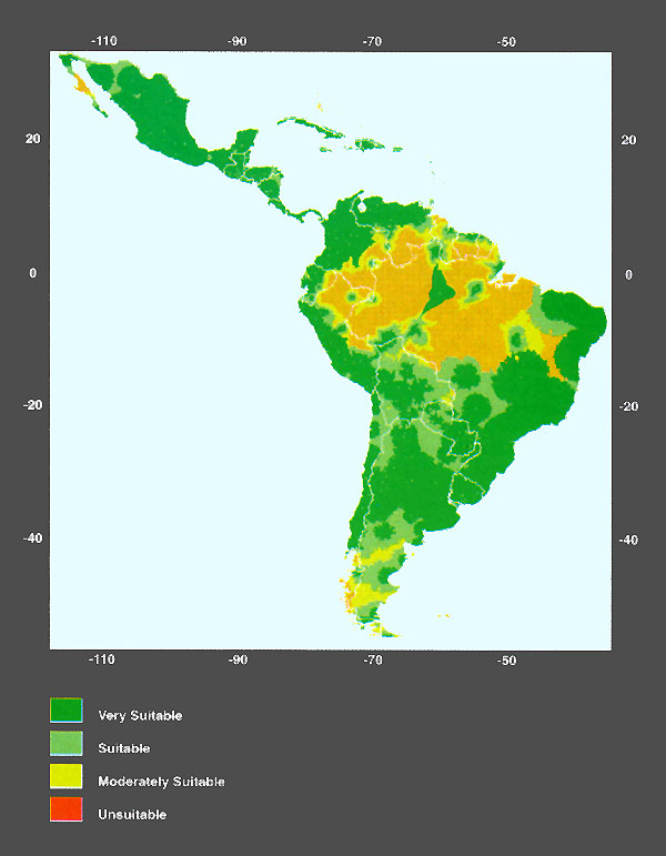
Figure 3.1
Potential market demand: commercial fish farming(mkt)
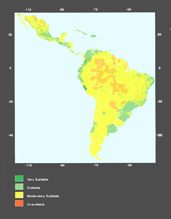
Figure 3.2
Potential for farm gate sales (fgs)
Figure 3.3
Soil and terrain suitability for ponds (sol)
Figure 3.4
Potential for agriculture by-products as feed and fertiliser inputs (croppot)
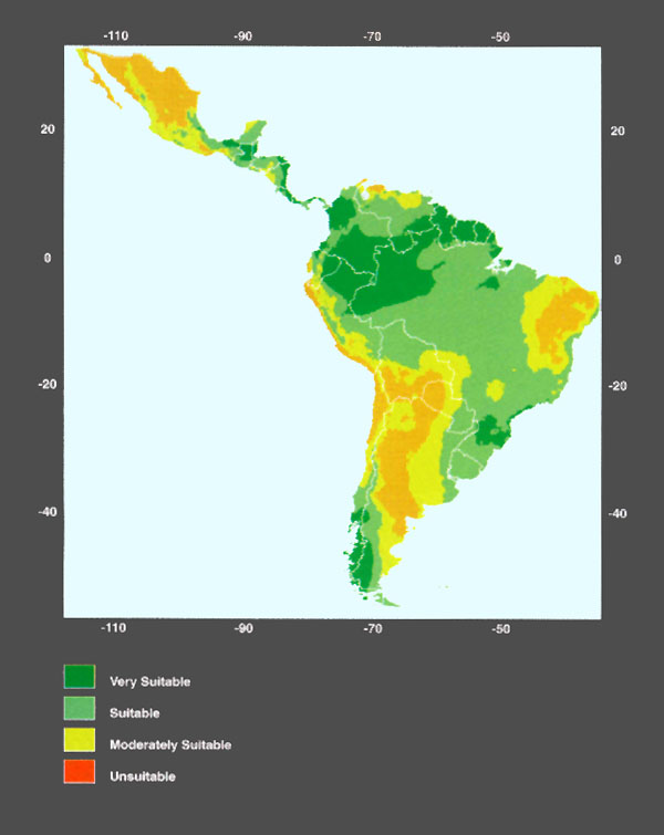
Figure 3.5
Net annual water loss from ponds through evaporation and seepage (evpseep)
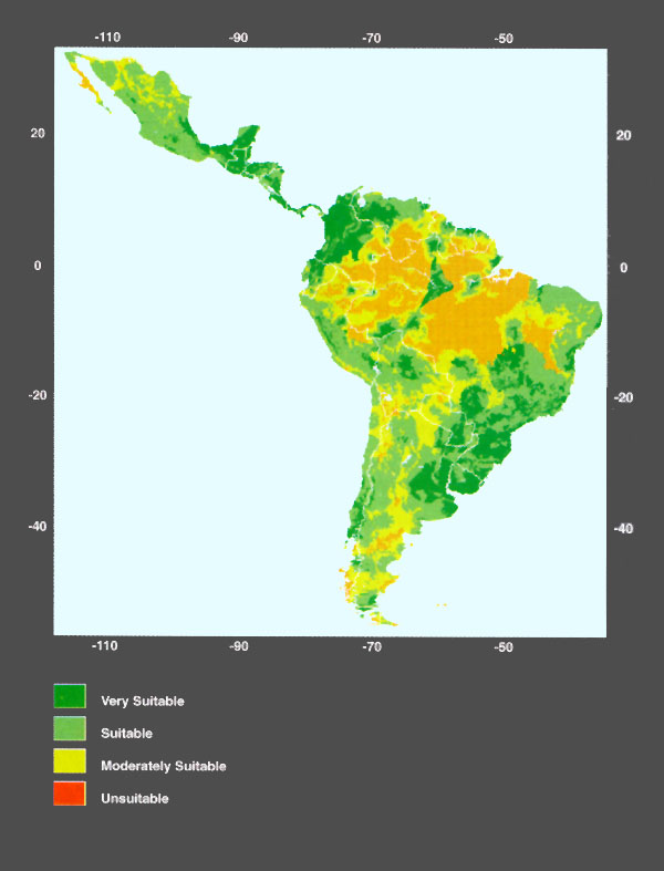
Figure 3.6
Suitability for commercial fish farming (com_mld)
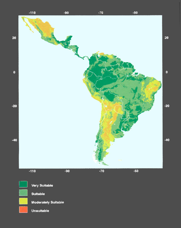
Figure 3.7
Suitability for small scale fish farming (sub_mld)
When the five factors discussed above are combined to make the commercial model, the result is that about 20% of Latin America scores VS, about 38% S and about 22% MS (Figure 3.6). For the small-scale model, about 31% of the continent scores VS, nearly 44% S and 15% MS (Figure 3.7). Central America, NW and SE South America are areas where both commercial and small-scale farming are favoured.
The effect of proximity to large urban centres can be clearly seen as circular areas on the map (Figure 3.1). Five countries, Belize, Costa Rica, El Salvador, Guatemala and Uruguay, have 100% or nearly 100% of their national areas scoring VS for this factor (Figure 3.8). Eleven other countries have from 50% to nearly 90% of their areas in this category. Only Suriname has a low overall score, with just over 50% of its area that is at least MS.
Only one country, El Salvador, has a large area (about 60%) that is VS for farm-gate sales, whereas most of the other countries have 5% or less of their area in this category (Figures 3.2 and 3.9). Only one country, Honduras, has more than half of its area that is suitable for farm-gate sales. There are six additional countries that have more than 25% of their national area classed as suitable.
Uruguay and Argentina respectively have about 25 and 20% of their area that scores VS (Figures 3.3 and 3.10). There are eleven countries that have 50% or more of their soil areas that score VS or S together. French Guiana and Guyana are notably relatively lacking in good quality soils for ponds.
Three countries, El Salvador, Suriname and Uruguay, have nearly one-half of their national areas that score VS for potential agricultural by-products, but most countries have much of their area that scores either S or MS for this factor (Figures 3.4 and 3.11). Chile is the only country with less than one-half of its national area that is not at least MS in potential for agricultural by-products.
Seven countries score VS for 50% or more of their areas and eight others have from 25 to 50% of their area that is VS (Figures 3.5 and 3.12). Mexico and Argentina stand out as countries with relatively small areas that score VS or S for water loss, suggesting that water requirements could be a relatively serious constraint there.
Figure 3.8 Potential Market Demand: Commercial Fish Farming
Figure 3.9 Potential for Farm Gate Sales
Figure 3.10 Soil and Terrain Suitability for Ponds
Figure 3.11 Potential for Agricultural By-Products as Feed and Fertliser inputs
Figure 3.12 Net Annual Water Loss from Ponds through Evaporation and Seepage
Figure 3.13 Suitability for Commercial Fish Farming
Generally, the countries of Central America, NW and SE South America are favoured in suitability for commercial farming (Figure 3.6). Three countries, Costa Rica, Belize and Guatemala, have more than 90% of their area classed VS for commercial farming (Figure 3.13). Six other countries have more than 50% of their national area that scores VS. For five of them, all, or most of the remaining area, is classed S. French Guiana and Suriname have relatively small areas that are VS or S, although these together have a combined total of more than 30%. Brazil has the least area that rates MS or better, although the combined total exceeds 60%.
Two countries, French Guiana and Suriname, have more than 90% of their area that is VS for small-scale farming and there are eight additional countries that have more than 50% of their area in the VS category (Figures 3.7 and 3.14). Additionally, for the same countries the remaining area is all S, or nearly so. Mexico is least favoured; although even there about 60% of the country is MS or better for small-scale farming, of which about 13% is VS and 25% S.
Figure 3.14 Suitability for Small-Scale Fish Farming
Yields in terms of crops/y are the key output from the growth model for the four different fish species. This output is presented first from a continental viewpoint and then from a country viewpoint. The continental country-level results are expressed in terms of relative surface area. For simplicity, crops/y results have been separated into quarter parts of the ranges that have been attained with each feeding rate × harvest weight combination. Again, for simplicity, only the first three quarters are presented as histograms, but all four quarters are mapped.
Relatively large areas of Latin America are suitable for the commercial farming of the four species considered here. For example, areas in which 1stQ (i.e., highest) crops/y are attainable range from a high of 74% of Latin America for carp to a low of about 36% for Nile tilapia, except for one result for the latter species that is only 11%. Results for individual species range from 67 to 74% for carp (Figure 3.15), 11 to 45% for Nile tilapia (Figure 3.16), 57 to 67% for tambaqui (Figure 3.17) and 49 to 61% for pacu (Figure 3.18).
Significantly, areas corresponding to 2ndQ and 3rdQ crops/y are small in comparison to 1stQ areas, except for the 50% satiation feeding rate of Nile tilapia (Figures 3.15 to 3.18). Therefore, most of the area that is apt for farming of these four species is capable of producing relatively high numbers of crops/y in each feeding rate × harvest weight combination.
Within individual species results, there is relatively little difference in the 1stQ surface areas that result from different feeding rate - harvest size combinations (Figures 3.15 to 3.18). Rather, it is the numbers of crops/y that vary markedly when the different regimes are simulated. As would be expected, it is the combination of low feeding rate and high harvest weight that tends to produce the least crops/y and conversely, the high feeding rate - low harvest weight that results in the highest number of crops/y. In general, feeding at the high rate (75%) provides a good combination of relatively large surface areas and high number of crops/y. Feeding at 50% and harvesting at the high weight clearly produces the lowest crops/y along with the least surface area, except for tambaqui, for which the lowest 1stQ area is obtained with 50% feeding and the low harvest size.
For small-scale farming, the results vary considerably between the two species considered. For Nile tilapia harvested at 150g, a relatively small area of Latin America (36%) can yield 1.3 to 1.7 crops/y and an additional 13% of the surface area can produce 0.9 to 1.3 crops/y (Figure 3.16). In contrast, 72% of the continent can produce 1.4 to 1.8 crops/y of carp harvested at 350g, and another 12% of the area can produce 0.9 to 1.4 crops/y (Figure 3.15).
Figure 3.15 Relative Surface Areas and Yield Ranges for Carp under Various Feeding Rate - Harvest Weight Combinations
Figure 3.16 Relative Surface Areas and Yield Ranges for Nile Tilapia under Various Feeding Rate - Harvest Weight Combinations
Figure 3.17 Relative Surface Areas and Yield Ranges for Tambaqui under Various Feeding Rate - Harvest Weight Combinations
Figure 3.18 Relative Surface Areas and Yield Ranges for Pacu under Various Feeding Rate - Harvest Weight Combinations
In this section we generalize the spatial distribution of species potential on a country by country basis. Each feeding rate - harvest weight combination is illustrated by a histogram. However, as indicated above, among feeding rate × harvest weight combinations within species there is relatively little surface area difference, with one exception in the case of the Nile tilapia. Further, it is difficult to discriminate such small area differences on the continental maps reduced to A4 size for this publication. For these reasons and also for economy in publication costs, only one map is used to illustrate the spatial distribution of each species. As has been shown above, it is the combination of feeding at 75% satiation with the low harvest weight that provides the highest numbers of crops/y along with relatively large surface areas. Therefore, this combination has been selected for the map illustration.
The spatial pattern for tambaqui is similar among the feeding rate - harvest weight combinations: 1stQ crops/y are possible in S Mexico and in all or nearly all of the national areas of the Central American countries south of Mexico, throughout the N and NW of South America apart from the Andes, over much of Brazil (apart from the SE) and parts of Bolivia, Paraguay and Peru (Figures 3.19 to 3.23). It is all but N Argentina, Chile, N Central Mexico and Uruguay that are disadvantaged.
The spatial pattern for pacu is similar to that of tambaqui; however, it is more restrictive in that 1stQ crops/y areas are less and 2ndQ crops/y areas are larger (Figures 3.24 to 3.28).
The spatial distribution of commercial culture opportunities for the Nile tilapia is markedly more restrictive than for the other species; however, the same group of Central American and N and NW South American countries maintain 1stQ crops/y potential, but much of the relatively high yield potential is lost in the marginal countries (Figures 3.29 to 3.33).
As would be expected for a species with a relatively wide temperature range for growth, the spatial distribution for carp culture is greater compared to the other species (Figures 3.34 to 3.38). For example, 1stQ and 2ndQ crops/y ranges can be realized over much of Mexico and in N. Argentina, whereas only small areas of these regions are apt for the other three species.
Carp and Nile tilapia contrast greatly in the spatial distribution of their small-scale-culture potential. Nile tilapia is apt for small-scale farming in the same countries as carp and 1stQ and 2ndQ crops/y ranges are similar to those of the carp, but Nile tilapia potential extends over a smaller area (Figures 3.41 and 3.42). Nevertheless, 1stQ crops/y (1.3 to 1.7) can be obtained in 50% or more of 11 countries, and only Uruguay and Chile offer no possibilities for yields in the 1stQ and 2ndQ ranges. Opportunities for small-scale farming of carp are extensive. 1stQ yields of from 1.4 to 1.8 crops/y can be attained in more than 50% of the areas of all but three of the countries and it is only Chile that is quite disadvantaged.
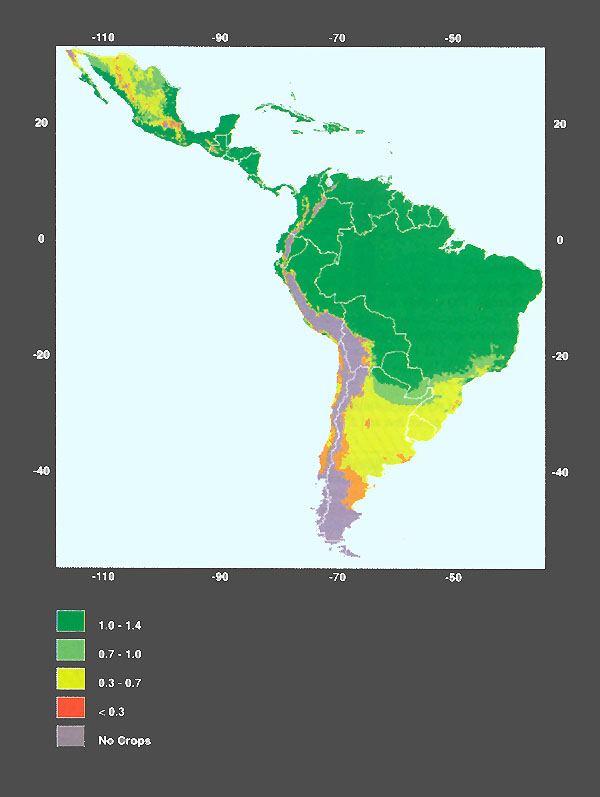
Figure 3.19
Potential yield (crops/y) of tambaqui fed at 75% satiation and harvested at 600 g (cc750600)
Figure 3.20 Relative Surface Area - Yield Combination for Tambaqui Fed at 75% Satiation and Harvested at 600g
Figure 3.21 Relative Surface Area - Yield Combination for Tambasqui Fed at 75% Satiation and Harvested at 1000g
Figure 3.22 Relative Surface Area - Yield Combination for Tambaqui Fed at 50 % Satiation and Harvested at 600 g
Figure 3.23 Relative Surface Area - Yield Combination for Tambaqui Fed at 50% Satiation and Harvested at 1000 g

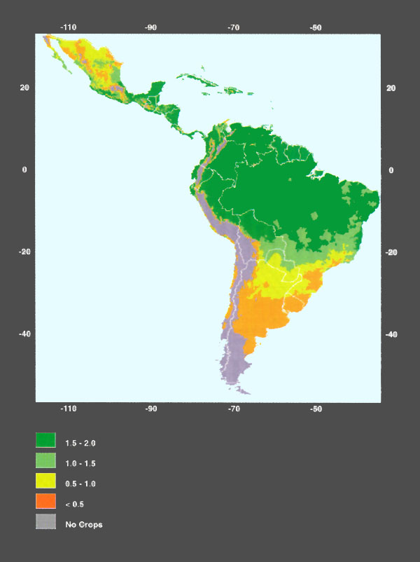
Figure 3.24
Potential yield (crops/y) of pacu fed at 75% satiation and harvested at 600 g (cp750600)
Figure 3.25 Relative Surface Area - Yield Combination for Pacu Fed at 75% Satiation and Harvested at 600 g
Figure 3.26 Relative Surface Area - Yield Combination for Pacu Fed at 75% Satiation and Harvested at 1000g
Figure 3.27 Relative Surface Area - Yield Combination for Pacu Fed at 50% Satiation and Harvested at 600g
Figure 3.28 Relative Surface Area - Yield Combination for Pacu Fed at 50% Satiation and Harvested at 1000g
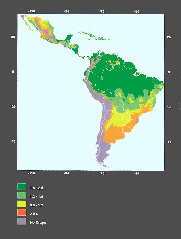
Figure 3.29
Potential yield (crops/y) of Nile tilapia fed at 75% satiation and harvested at 300 g (ct750300)
Figure 3.30 Relative Surface Area - Yield Combination for Nile Tilapia Fed at 75% Satiation and Harvested at 300g
Figure 3.31 Relative Surface Area - Yield Combination for Nile Tilapia Fed at 75% Satiation and Harvested at 600g
Figure 3.32 Relative Surface Area - Yield Combination for Nile Tilapia Fed at 50% Satiation and Harvested at 300g
Figure 3.33 Relative Surface Area - Yield Combination for Nile Tilapia Fed at 50% Satiation and Harvested at 600g
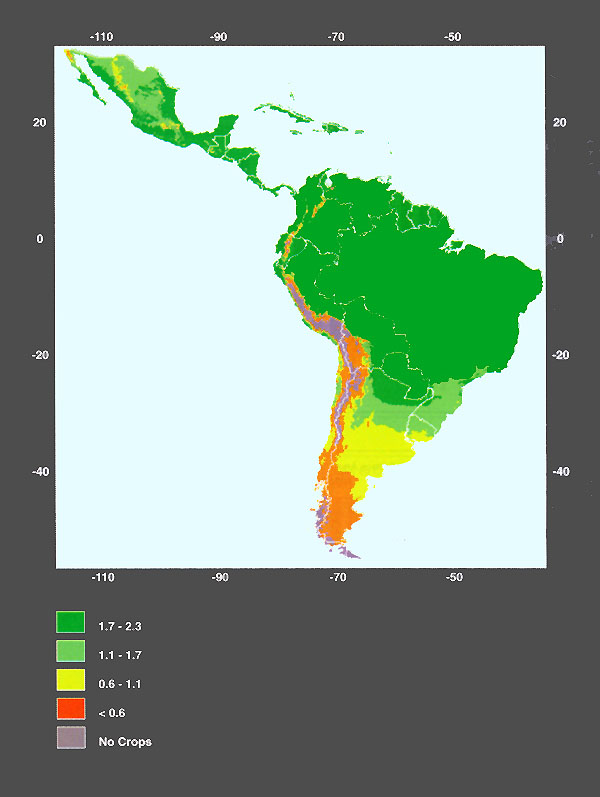
Figure 3.34
Potential yield (crops/y) of carp fed at 75% satiation and harvested at 600 g (cr750600)
Figure 3.35 Relative Surface Area - Yield Combination for Carp Fed at 75% Satiation and Harvested at 600g
Figure 3.36 Relative Surface Area - Yield Combination for Carp Fed at 75% Satiation and Harvested at 1500g
Figure 3.37 Relative Surface Area - Yield Combination for Carp Fed at 50% Satiation and Harvested at 600g
Figure 3.38 Relative Surface Area - Yield Combination for Carp Fed at 50% Satiation and Harvested at 1500g
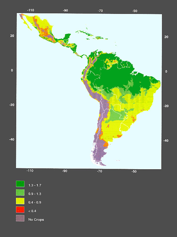
Figure 3.39
Potential yield (crops/y) of Nile tilapia with a CFB of 0.075 kg/M3 and harvested at 150 g (ct000150)
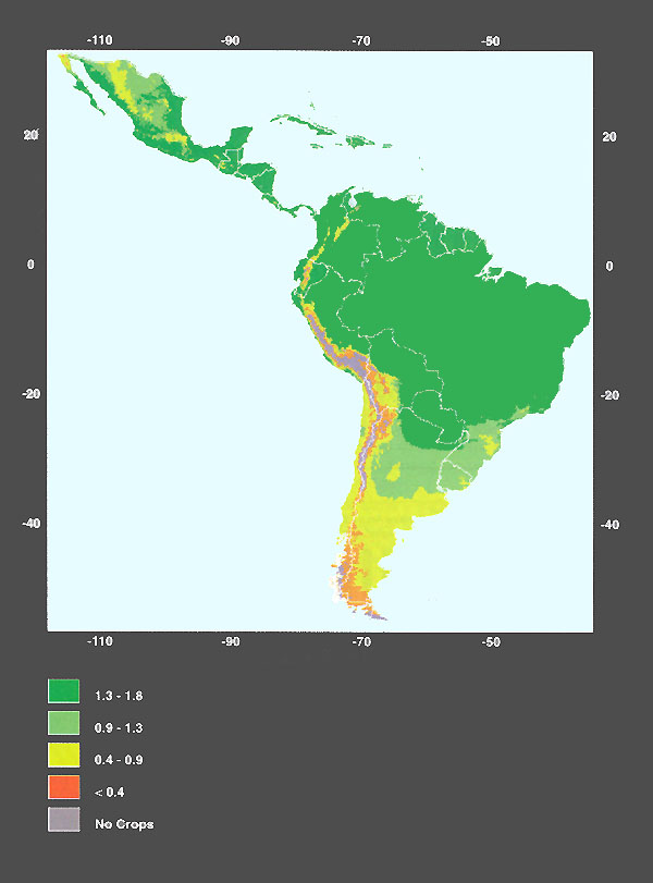
Figure 3.40
Potential yield (crops/y) of carp with a CFB of 0.075 kg/M3 and harvested at 350 g (cr000350)
Figure 3.41 Relative Surface Area - Yield Combination for Nile Tilapia with a CFB of 0.075 kg/m3 and Harvested at 150g
Figure 3.42 Relative Surface Area - Yield Combination for Carp with a CFB of 0.075 kg/m3 and Harvested at 350g
In this section we examine species yield potential as influenced by the five factors that affect the development and operation of fish farming in ponds after they have been brought together in the commercial model and four of the same factors which have been combined in the small-scale model. In order to draw attention to those areas of Latin America where conditions are most favourable for inland fish farming, as well as for simplicity and clarity, we discuss the spatial aspects of only the highest ranking combinations: areas that score VS or S for the commercial model and areas that are apt for fish crops in the 1stQ and 2ndQ ranges of crops/y. However, the maps do indicate all of the combinations of model outcomes from VS to MS, and crops/y outcomes for the 1stQ, 2ndQ and 3rdQ ranges.
Even with the constraints imposed by meeting the factor requirements of the commercial model along with those of favourable water temperatures, there are large areas of Latin America that are very apt for commercial fish farming of the four species under consideration herein. Area-wise, the pattern shows very little difference among feeding rate × harvest weight combinations within species (Figures 3.43 to 3.46). Among species, areas that score S-2ndQ to VS-1stQ range from a low of 19 to 25% for the Nile tilapia, from 25 to 35% for pacu, from 33 to 36% for tambaqui, and up to 40 to 44% for carp. This suggests that, in terms of areas suitable, opportunities for carp farming are considerably better than for Nile tilapia, while tambaqui and pacu are intermediate.
As would be expected, the pattern established earlier - suggesting that the high feeding rate combined with the low harvest weight provides the largest area, and also the highest number of crops/y - also holds when the commercial model is brought in. However, as noted above, the range of differences in areas among the various feeding rate × harvest weight combinations is not great.
Within the small-scale model, 60% of continental Latin America is very apt for farming of carp and will provide 0.9 to 1.8 crops/y (Figure 3.46). About 24% of that area scores VS and could provide from 1.4 to 1.8 crops/y.
In contrast, the area that is very apt for Nile tilapia small-scale farming and which will provide 0.9 to 1.7 crops/y is about 38%. About 16% of this area scores VS and could provide 1.3 to 1.7 crops/y (Figure 3.43).
As was pointed out above, there is little spatial difference from one feeding rate × harvest weight strategy to another within a species. Thus, the spatial distribution can be adequately illustrated by a single map for each species. We have chosen the high feeding rate × low harvest weight combination map for each species because, as already established, this strategy results in the highest crops/y over the largest expanses of area. However, histograms of the spatial distribution pertaining to each feeding rate × harvest weight combination are presented.
Tambaqui
The countries most favoured for the commercial farming of this species are all in Central America (Figures 3.47 to 3.51). There are six countries that have more than 50% of their area that scores VS-1stQ (1.1 to 1.4 crops/y) for the 75%-600g combination. Eleven additional countries have at least 30% of their areas that provide a minimum of S-2ndQ possibilities.
Pacu
The results for this species are nearly identical to those for tambaqui in terms of spatial distribution and rank order of the countries in area (Figures 3.52 to 3.56), but for the 75%-600g combination, higher yields, of 1.5 to 2 crops/y, are included in the 1stQ range of crops/y.
Carp
As with tambaqui and pacu, Central American countries score high, with more than 40% of the national area being VS-1stQ (1.7 to 2.3 crops/y) for the 75%-600g combination. However, other countries possess relatively large areas that provide at least S-2ndQ possibilities, among them Mexico and Uruguay (Figures 3.57 to 61).
Nile tilapia
Although the Central American countries dominate, the areas that score highest are considerably less than for the other species (Figures 3.62 to 3.66). There are only three countries, Belize, Costa Rica and El Salvador, that have more than 50% of their area classed VS-1stQ (1.8 to 2.4 crops/y in the 75%-300g combination) and only one other, Panama, has in excess of 40% of its area that falls in the same category. Nevertheless, there are 11 additional countries that equal or exceed S-2ndQ possibilities over more than 30% of their national areas.
Unlike commercial-level farming, two of the northern South American countries - French Guiana and Suriname - score highest both for Nile tilapia and carp farming, and the ranks for the remaining countries are quite similar between the two species (Figures 3.67 to 3.70). Eight countries have more than 50% of their area that is VS-1stQ (1.4 to 1.8 crops/y) for carp harvested at 350g, whereas there are only one-half that number for Nile tilapia harvested at 150 g in the same category (1.3 to 1.7 crops/y). In all, there are 20 countries that meet or exceed S-2ndQ requirements for over 20% or more of their national areas for carp and 18 for Nile tilapia. Eight of these countries have more than 80% of their rated areas in this category for carp and 5 countries for Nile tilapia.
Figure 3.43 Relative Surface Areas with Suitability for Commercial and Small Scale for Farming and Yield Ranges for Nile Tilapia under Various Feeding Rate - Harvest Weight Combinations
Figure 3.44 Relative Surface Areas with Suitability for Commercial Farming and Yield Ranges for Pacu under Various Feeding Rate - Harvest Weight Combinations
Figure 3.45 Relative Surface Areas with Suitability for Commercial Farming and Yield Ranges for Tambaqui under Various Feeding Rate - Harvest Weight Combinations
Figure 3.46 Relative Surface Areas with Suitability for Commercial and Small Scale Farming and Yield Ranges for Carp under Various Feeding Rate - Harvest Weight Combinations
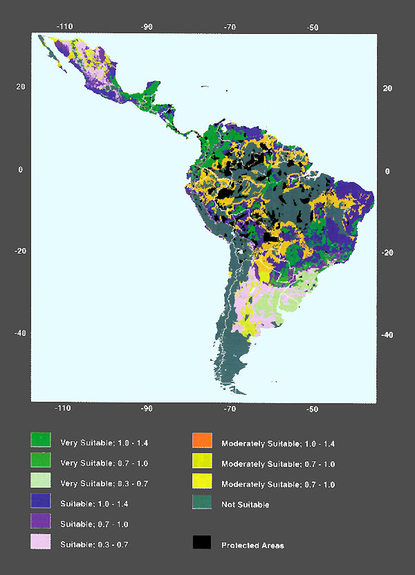
Figure 3.47
Suitability for commercial farming and potential yield (crops/y) of tambaqui fed at 75% satiation
and harvested at 600 g (mc750600)
Figure 3.48 Relative Surface Area with Suitability for Commercial Farming and Yield Range Combined for Tambaqui Fed at 75% Satiation and Harvested at 600g
Figure 3.49 Relative Surface Area with Suitability for Commercial Farming and Yield Range Combined for Tambaqui Fed at 75% Satiation and Harvested at 1000g
Figure 3.50 Relative Surface Area with Suitability for Commercial Farming and Yield Range Combined for Tambaqui Fed at 50% Satiation and Harvested at 600g
Figure 3.51 Relative Surface Area with Suitability for Commercial Farming and Yield Range Combined for Tambaqui Fed at 50% Satiation and Harvested at 1000g
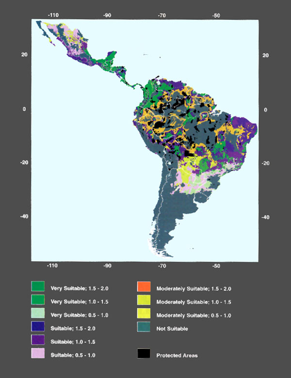
Figure 3.52
Suitability for commercial farming and potential yield (crops/y) of pacu fed at 75% satiation
and harvested at 600 g (mp750600)
Figure 3.53 Relative Surface Area with Suitability for Commercial Farming and Yield Range Combined for Pacu Fed at 75% Satiation and Harvested at 600g
Figure 3.54 Relative Surface Area with Suitability for Commercial Farming and Yield Range Combined for Pacu Fed at 50% Satiation and Harvested at 1000g
Figure 3.55 Relative Surface Area with Suitability for Commercial Farming and Yield Range Combined for Pacu Fed at 50% Satiation and Harvested at 600g
Figure 3.56 Relative Surface Area with Suitability for Commercial Farming and Yield Range Combined for Pacu Fed at 50% Satiation and Harvested at 1000g
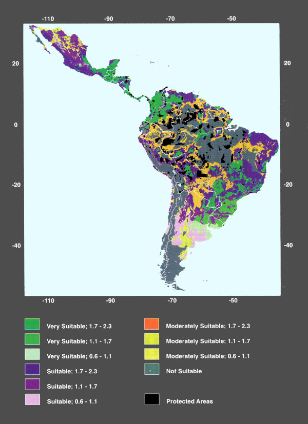
Figure 3.57
Suitability for commercial farming and potential yield (crops/y) of carp fed at 75% satiation
and harvested at 600 g (mr750600)
Figure 3.58 Relative Surface Area with Suitability for Commercial Farming and Yield Range Combined for Carp Fed at 75% Satiation and Harvested at 600g
Figure 3.59 Relative Surface Area with Suitability for Commercial Farming and Yield Range Combined for Carp Fed at 75% Satiation and Harvested at 1500g
Figure 3.60 Relative Surface Area with Suitability for Commercial Farming and Yield Range Combined for Carp Fed at 50% Satiation and Harvested at 600g
Figure 3.61 Relative Surface Area with Suitability for Commercial Farming and Yield Range Combined for Carp Fed at 50% Satiation and Harvested at 1500g

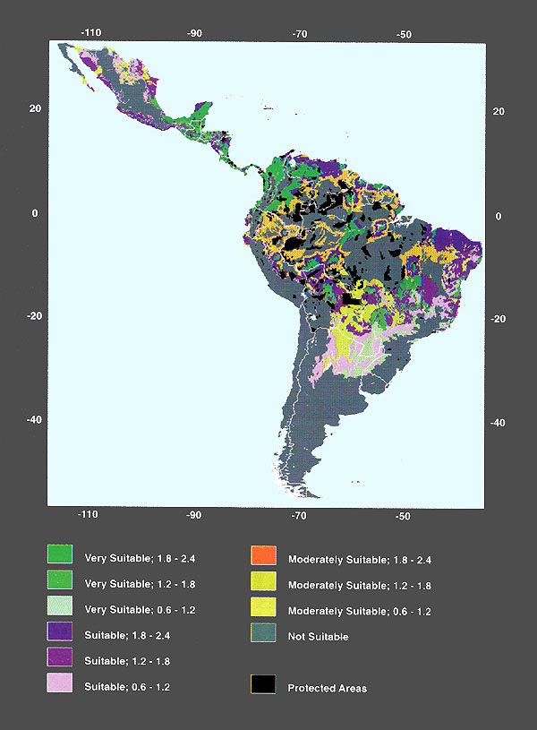
Figure 3.62
Suitability for commercial farming and potential yield (crops/y) of Nile tilapia fed at 75% satiation
and harvested at 300 g (mt750300)
Figure 3.63 Relative Surface Area with Suitability for Commercial Farming and Yield Range Combined for Nile Tilapia Fed at 75% Satiation and Harvested at 300g
Figure 3.64 Relative Surface Area with Suitability for Commercial Farming and Yield Range Combined for Nile Tilapia Fed at 75% Satiation and Harvested at 600g
Figure 3.65 Relative Surface Area with Suitability for Commercial Farming and Yield Range Combined for Nile Tilapia Fed at 50% Satiation and Harvested at 300g
Figure 3.66 Relative Surface Area with Suitability for Commercial Farming and Yield Range Combined for Nile Tilapia Fed at 50% Satiation and Harvested at 600g
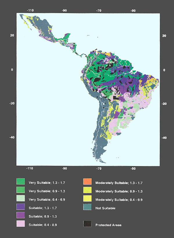
Figure 3.67
Suitability for small scale farming and potential yield (crops/y) of Nile tilapia with a CFB of 0.075 kg/ m3
and harvested at 150 g (mt000150)
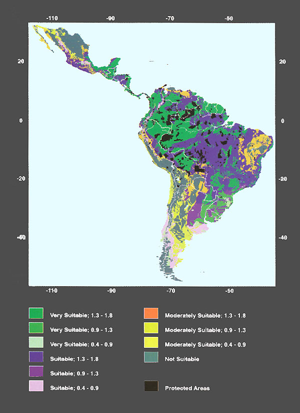
Figure 3.68
Suitability for small scale farming and potential yield (crops/y) of carp with a CFB of 0.075 kg/ m3
and harvested at 350 g (mr000350)
Figure 3.69 Relative surface Area with Suitability for Commercial Farming and Yield Range Combined for Nile Tilapia with a CFB of 0.075 kg/m3 and Harvested at 150g
Figure 3.70 Relative Surface Area with Suitability for Commercial Farming and Yield Range Combined for Carp with a CFB of 0.075 kg/m3 and Harvested at 350g
This section compares the predictions of suitability for commercial fish farming and predicted yield potential with observations from 34 commercial fish farms in Colombia.
All of the 34 farms raised red tilapia (tilapia roja) alone or predominately (Table 3.2). Nearly all farms were using semi-intensive or intensive methods (Table 3.3).
The weights at harvest of red tilapia among 32 commercial farms averaged 405 g and the median was 378 g (Table 3.4).
Thus, considering species cultured, intensity of farming and harvest weight, the most appropriate grid cell “site” comparison with farm locations corresponded to the predicted potential for commercial farming of Nile tilapia fed at 75% satiation and harvested at 300 g.
The outcome of this comparison was that 20 of the farms were in grid cells predicted to be VS by the commercial model, of which 13 farms were in cells predicted to yield crops in the 1stQ range, four in the 2ndQ range and three in the 3rdQ range. Fourteen farms were in grid cells either US from the viewpoint of the commercial model, or with crops/y falling into the 4thQ range (Table 3.5).
Table 3.2 Farms raising red tilapia, cachama and other species among those surveyed.
| No. of farms | Species mix |
|---|---|
| 10 | Tilapia roja alone |
| 20 | Tilapia roja with cachama alone, or with others |
| 3 | Tilapia roja with others, but not cachama |
| 1 | No data |
| 34 | Total |
Table 3.3 Intensity of farming among 32 farms
| No. of farms | Intensity of farming |
|---|---|
| 1 | Extensive |
| 23 | Semi-intensive |
| 8 | Intensive |
| 2 | No data |
| 34 | Total |
Table 3.4 Weights at harvest of red tilapia from 32 commercial farms in Colombia
| Weight at harvest of red tilapia (g) | Number of farms |
|---|---|
| 201–250 | 4 |
| 251–300 | 5 |
| 301–350 | 4 |
| 151–200 | 1 |
| 351–400 | 5 |
| 401–450 | 2 |
| 451–500 | 7 |
| 501–550 | 1 |
| 551–600 | 2 |
| > 600 | 1 |
| No data | 2 |
Table 3.5. Predicted suitability of grid cell sites containing 34 fish farms for commercial farming of Nile tilapia fed at 75% satiation and harvested at 300 g
| Score for the commercial model | Score for yield in crops/y (quarter ranges) | Number of farms |
|---|---|---|
| VS | 1st Q | 13 |
| VS | 2nd Q | 4 |
| VS | 3rd Q | 3 |
| US (i.e., US for the commercial model, or crops/y in 4th Q) | 14 | |
For the purposes of verification, it is most important to know why the predictions of commercial suitability and yield potential did not correspond to the locations of the active commercial fish farms so that future versions of the models can be refined. Therefore, the 14 farms locations that were US for Nile tilapia were the focus of subsequent investigations.
In order to further pin down the causes for the disparity at the 14 US grid cell sites, the 34 farm locations were compared with predictions of suitability made by the commercial model alone. The outcome was that all the sites that were US (Table 3.5) were, in fact, VS for the commercial model. Therefore, the apparent problem at the commercial farm locations was not with any of the factors upon which the commercial model is based, but with the growth model that predicts yield in crops/y. Because the most important input factor of the yield model is the mean monthly temperature regime, possible temperature anomalies at the 14 farm locations were investigated.
In order to test the hypothesis of temperature anomalies, the 34 farm locations were compared with the predicted for carp fed at 75% satiation and harvested at 600 g. It was reasoned that, if the problem is indeed one of temperature, then more farm locations should be suitable for carp than for Nile tilapia because the former species is more tolerant to lower temperatures than the latter.
The outcome of this comparison was that all but one site was in the 1stQ range of crops/y for carp and the remaining site was in the 2ndQ range. This suggests that, indeed, the problem is related to temperature at the 14 fish farm locations US for Nile tilapia. With regard to the predictions of tilapia yields, the problem can have three sources:
predicted water temperatures are lower than actual temperatures,
the model is not adjusted to reflect actual farming conditions with respect to water temperature, or
the mainly red tilapia strains grown in Colombia are more cold tolerant than those upon which the model is based.
Predicted vs actual temperatures
One way that predicted temperatures for grid cells can be lower than actual temperatures at farm sites is related to the terrain and grid cell size in relation to farm size. The nominal dimensions of a grid cell are 9 × 9 km, or 81 km2 whereas the farms are a fraction of this area (Table 3.6), as half of the 34 commercial farms were less than 5 ha in extent.
Table 3.6 Commercial farm sizes among a sample of 34 in 8 departmentos in Colombia
| Size Interval (ha) | Number of Farms |
|---|---|
| 1–5 | 17 |
| 6–10 | 7 |
| 11–15 | 3 |
| 16–20 | 3 |
| 21–25 | 1 |
| 26–30 | 1 |
| > 30 | 2 |
| Total | 34 |
The water temperature predicted for a grid cell characterises its entire area based on air temperature which, in turn, is partly based on altitude. Another way of expressing the same idea is that farms inhabit a microclimate compared to the “macroclimate” of the grid cell in which they are located. This hypothesis was tested by examining the terrain in the vicinity of the fish farms that were US for Nile tilapia, mainly using 1:25 000 scale maps, or else 1:100 000 maps.
As would be expected, in the hilly and mountainous terrain of W Colombia, nearly all of farms are located on relatively flat land in valleys. To generalize, of those that were US, many are in the range of 600–1 000 m and there are altitudes of from 1 300 m up to 3 000 m within relatively short distances of about 4 to 10 km from them. Two of the farms that were US are at about 1 350 and 1 500 m. Thus, it is highly likely that, because of the surrounding terrain, the estimated temperatures of the grid cells in which the farms fall are less than the actual temperatures at the farm sites.
In order to test the general correspondence between predicted and observed water temperatures, the grids of mean monthly temperature were queried for the grid cells with temperature observations and also grid cells encompassing the locations of the three fish farms (labelled F1, F2 and F3 respectively) that were both US for tilapia and at the highest altitudes. The water temperatures reported for Farms 1, 2 and 3 were in the ranges of 21–30°, 20–27° and 23–25°C, respectively. In comparison, predicted temperatures for the same locations ranged from 22.2–23.4°, 19.8–21.4° and 22.4–23.7°C. These data suggest a tendency towards both lower values and a narrower range for predicted temperatures, which may in part account for poor predictions of Nile tilapia yields in the grid cells where active farms exist.
Another aspect of this same problem is that predicted water temperatures were based only on actual air temperature inputs; other model inputs were from our weather generator, which gives “reasonable” guesses at best.
Different strains of tilapia being grown on the farms
It is possible that the mainly red tilapia strains used at the locations are either more cold-tolerant than “typical Nile tilapia” or have adapted to ambient conditions on the farms. For example, cold-adapted strains of Nile tilapia from Egypt were successfully grown at high altitudes and low temperatures in Rwanda (Nathanael and Moehl, 1989).
Model parameters
The lower temperature threshold in the growth model is about 18.6°C for Nile tilapia. Model parameters were based on growth data from Honduras (see Annex 2). This lower threshold may be a little too high because Nile tilapia is capable of survival, if not growth, at temperatures as low as about 16°C. However, we settled on a lower threshold of 18.6°C because it provided reasonable predictions of yields in locations as diverse as El Carao, Honduras, and Bangkok, Thailand, during the model validation phase (see Annex 2).
![]()
![]()
![]()