![]()
![]()
![]()
From these sources and the Appendix maps, the following compressed summary was constructed.
CALIFORNIA CURRENT SYSTEM
Columbia River. Anchovy spawning region (only in summer, moderate biomass); moderate continental shelf width; intense wind-generated turbulent mixing, relaxing during summer; stable upper ocean structure during summer due to lens of fresh water at the surface; onshore Ekman transport during winter--weak offshore Ekman transport during summer; little onshore-offshore temperature contrast except very near the coast.
Cape Mendocino. Primary upwelling center; narrow continental shelf; intense offshore Ekman transport, except in winter; intense turbulent mixing throughout the year; intense summer cold coastal temperature anomaly; small biomass of locally spawning fish populations; feeding grounds of adult pelagic fishes spawning elsewhere.
Southern California Bight. The major spawning grounds of pelagic fishes of the California Current; anchovy spawning region (entire year, peaking in winter-spring; large biomass); sardine spawning region (spring, pre-collapse landings 800,000 t); weak offshore Ekman transport; wide continental shelf; moderately weak turbulent mixing; relatively stable upper ocean density structure; warm coastal temperature anomalies extending very near to coast; semi-enclosed inshore gyral circulation pattern.
Punta Baja. Secondary upwelling center; narrow continental shelf; strong offshore Ekman transport, peaking in spring; moderate wind-generated turbulence; lies between two gyral circulations to the north and south and divides areas occupied by separate subpopulations of pelagic fishes. Some spawning occurs (often regarded as contiguous with Southern California Bight spawning populations). Weak negative coastal temperature anomaly.
Southern Baja California. Anchovy spawning region (winter-spring peak, moderate biomass); sardine spawning region (entire year, spring peak--moderate biomass); moderate continental shelf width; strong offshore Ekman transport; weak to moderate turbulent mixing; relatively stable upper ocean density structure; tendency for gyral circulation pattern; warm coastal temperature anomaly.
PERU CURRENT SYSTEM
Chimbote. Anchovy spawning region (spring peak, very large pre-collapse biomass); sardine spawning region (winter-spring); wide continental shelf; strong offshore Ekman transport and up- welling; weak wind-generated turbulence; very intense coastal cooling.
San Juan. Upwelling center; intense offshore Ekman transport, particularly in winter; narrow continental shelf; Turbulence level is low in summer, moderate in winter. Less stable stratification than in adjoining areas; very intense coastal cooling; reduced spawning of pelagic fishes relative to neighboring coastal areas (anchovy spawning appears to be intermediate in timing between Chimbote and Africa).
Africa. Anchovy spawning area (winter peak, large pre-collapse biomass); sardine spawning region (winter peak, large biomass); very low turbulence; weak offshore Ekman transport; moderate shelf width; extensive warm coastal temperature anomaly with a narrow band of cooling directly adjacent to the coast; gyral coastal circulation pattern.
Coquimbo. Upwelling center; intense offshore Ekman transport; extremely narrow continental shelf; cold coastal temperature anomalies extending hundreds of kilometers offshore. Turbulence level is moderate in summer, high in winter. No reported pelagic fish spawning.
Talcahuano. Seasonal upwelling (summer); moderate continental shelf width; turbulence level highest in spring; definite spatial minimum in fall and winter turbulence distributions. Anchovy spawning is reported (fall and winter only). Sardine eggs have been found.
46°S. Extreme wind-generated turbulent mixing--much higher than at the same latitude in the California Current region; no reported anchovy or sardine spawning.
CANARY CURRENT SYSTEM
Lisbon. Moderate upwelling; moderate to high wind-generated turbulence; moderately cool coastal temperature anomaly; moderate continental shelf width.
Casablanca. Sardine spawning region (peak in winter; secondary peak in summer); low turbulence levels (maximum in spring); low Ekman transport; moderate continental shelf width; slightly warm coastal temperature anomaly.
Cap Sim. Upwelling center (strongest offshore Ekman transport in summer); high wind-generated turbulence (minimum in fall); cold coastal temperature anomaly (intense in summer).
Ifni. Sardine spawning region (peak in winter, secondary peak in summer); moderate offshore Ekman transport (strongest in summer); moderate continental shelf width—shelf widens to the immediate south; local minimum in wind generated turbulence.
Cabo Bojador. Strong summer offshore Ekman transport—moderate offshore transport during the remainder of the year; fairly narrow continental shelf; turbulence levels moderate to high (summer maximum); substantial cold coastal temperature anomaly.
Cap Blanc. Upwelling center (intense offshore Ekman transport throughout the year); moderate continental shelf width; strong negative coastal temperature anomaly; moderate turbulent mixing in winter—stronger in summer.
Cap Vert. Highly seasonal upwelling; strong offshore Ekman transport in winter, relaxing greatly in summer; turbulence levels low in late summer and in fall—high in winter and spring; cold coastal temperature anomaly in winter—warm anomaly in summer. Summer and fall temperature exceed 27°C.
BENGUELA CURRENT SYSTEM
Cape Frio. Upwelling center; intense offshore Ekman transport throughout the year, extreme in winter to early spring; strong coastal temperature gradients.
Palgrave Point. Anchovy and sardine spawning grounds (summer); substantial offshore Ekman transport (although much weaker than in the adjacent regions to the north and south--weakest in the summer); fairly wide continental shelf; weak to moderate turbulent mixing--weakest in summer (definite local minimum in the spatial distributions of wind-generated mixing energy production); stable density structure in summer.
Lüderitz. Upwelling center; very intense offshore Ekman transport; moderately narrow continental shelf; intense turbulent mixing—peak intensity in summer; intense cold coastal temperature anomaly throughout the year; low stability in the water column.
Cape Columbine. Sardine spawning grounds (summer--some anchovy spawning); seasonal upwelling; strong offshore Ekman transport in summer, vanishing in winter; moderate continental shelf width; moderate to strong turbulent mixing (spring maximum, fall minimum). A local minimum of turbulent mixing energy production lies within the coastal indentation just to the north of the cape.
Cape Agulhas. Anchovy and sardine spawning grounds (spring-summer); onshore Ekman transport; wide continental shelf; intense turbulent mixing, moderating somewhat in summer; stable ocean structure resulting from a thin lens of warm clear surface water from the Indian Ocean which overlies denser, more productive waters at depth (50–75 m).
PATTERN RECOGNITION
Our analyses of the climatological fields and information on spawning grounds suggest the following patterns. Upwelling centers, characterized by strong offshore Ekman transport, intense wind-generated turbulent mixing, reduced water column stability, and narrow continental shelves appear to be areas in which anchovies and sardines do not spawn. Spawning grounds tend to lie in coastal indentations where wind induced transport and turbulence are reduced and continental shelf width tends to be greater. The spawning grounds of the largest populations tend to be located downstream (equatorward) of upwelling centers. Smaller populations (e.g., Columbia River, Talcahuano) are located at the poleward extreme of upwelling regions where the upwelling is highly seasonal, and spawning occurs when various circumstances may reduce the effects of offshore transport and of mixing of the surface layers by the wind.
Temperature
Sea surface temperature is a better index for establishing cold temperature tolerance than warm temperature tolerance (i.e., it is a good index of the warmest water available but colder water is always available at greater depths). The physiological response of pilchard and anchovy eggs and larvae are best known for the stocks which spawn in the Southern California Bight. Lasker (1964) has shown that pilchard eggs and larvae developed normally between 13° and 21°C; however, larval mortality increased in experiments below 14°C. Incubation time decreased with increasing temperature and early growth was greatest at 16°endash;17°C. Anchovy eggs and larvae developed normally at 11°C (Lasker, 1964) and early growth was greatest at 21°C in the laboratory (Kramer and Zweifel, 1970).
As long as it does not approach the physiological limits, ambient temperature, at least in so far as it is reflected in sea surface temperature distributions (Table 4 and Appendix Charts 3 and 4), does not appear to exert any obvious control on reproductive habits. For example, seasonal spawning peaks off Southern Baja California and Cape Agulhas correspond to bimonthly temperature values of nearly 19°C, while at Talcahuano peak anchovy spawning occurs in winter at 13°C, even though warmer conditions are available at other seasons. Certainly, temperature conditions exceeding physiological tolerances would preclude occurrence. For example, it is probable that no anchovy spawning would occur in winter off the Columbia River (i.e., at 9°C) even if other conditions were favorable. However, in the regions where the temperatures are within physiological limits, the particular temperature appears not to be a dominant factor in determining spawning habits.
Turbulence
Spawning rarely occurs in areas of strong turbulent mixing of the upper water column. Spawning grounds are characterized by weak to moderate values of the mean cube of the wind speed, which is an index of the rate of addition of wind-generated turbulent energy to the water column (Husby and Nelson, 1982). Spawning grounds generally lie directly within spatial minima in the W3(wind speed cubed) distributions (Appendix Charts 9 and 10). Spawning habitats are characterized by increased stability in the internal density structure of the upper water column (Table 5, Fig.8) that would resist dispersion of fine-scale food strata by turbulence events related to storms.
Where spawning grounds occur in regions of moderate wind-generated turbulence, other factors influencing stability may be favorable to spawning. For example, off the Columbia River the anchovy population spawns only in the summer (i.e., directly out of phase with other California Current anchovy populations). At this season, the W3 index falls to moderate values (Fig. 7) and the subsurface stability is enhanced by the thin lens of less dense Columbia River Plume water at the sea surface. At Talcahuano, where turbulence conditions are not greatly lessened during summer, anchovy spawning remains generally in phase with other Peru Current populations; reference to Appendix Charts 9 and 10 will show that turbulent mixing in coastal areas north of Talcahuano is actually less in the winter downwelling season than in the summer upwelling season. Off Cape Agulhas, both anchovy and pilchard populations spawn under conditions characterized by substantial wind-generated mixing. However, this is a situation where particularly strong internal water column stability builds during the summer spawning season (Fig. 8), which may be due to an influx of warm Indian Ocean surface water (Darbyshire, 1966).
Transport
Areas of intense offshore transport conditions, where reproductive products might be lost from the vicinity of the coast, are characterized by minimum spawning of anchovies and pilchards. In many cases, the effects of transport and turbulence are confounded since strong wind driven offshore transport and strong wind-generated turbulence tend to coincide in eastern boundary upwelling systems. However, adaptations which result in the avoidance of offshore loss of reproductive products appear to be very widespread in fish species successfully inhabiting the California Current region (Parrish et al., 1981), indicating that transport must exact an important control on reproductive success. Note that in two situations where spawning takes place under relatively strong turbulent conditions (i.e., Talcahuano and Cape Agulhas) surface Ekman transport is directed onshore. In addition, Shelton and Hutchings (1982) have shown that a coastal jet between Cape Agulhas and Cape Columbine aids transport of larvae from the spawning grounds to the inshore nursery grounds. At Chimbote an enormous anchovy population has spawned in a situation characterized by strong offshore transport (Fig. 7); this situation is discussed in detail below.
DISCUSSION
The information presented in this analysis suggests that temperature, transport, and turbulence patterns greatly influence the timing and location of spawning grounds of anchovies and pilchards in eastern boundary currents. Furthermore no single feature has overriding control. It appears that individual stocks have adapted their reproductive strategies to achieve local optimum solutions to these three physical factors. We assume that this also applies to the three factors of the IREX equation which we have not addressed: food, predation, and population density. The question of how good individual optimum solutions are, is probably best judged by the size of the stocks.
The four major eastern boundary currents have a great deal in common. The locations and seasonality of maximum offshore Ekman transport appear to be closely related to the seasonal latitudinal shifts of the atmospheric pressure systems, intensification of the large-scale pressure gradients, and the relationships between these systems and the large-scale topography of the continents. However, as can be seen in the environmental features presented here, there are also large differences among them. For example, all four systems have maximum cold inshore-offshore temperature anomalies associated with summer maxima of offshore Ekman transport. These summer “maximum upwelling regions” have anchovy and/or sardine stocks with spawning grounds poleward and equatorward of them. The California and Benguela systems each have a single area with cold sea surface temperature anomalies. In the California system this area is located in the summer upwelling maximum, whereas the Benguela system's area includes the summer upwelling maximum at Lüderitz and a winter upwelling maximum at Cape Frio. The Peru and Canary systems each have two separate areas of cold sea surface temperature anomalies. The Peru system has an area located at the winter upwelling maximum (San Juan to Chimbote) and a second area in the upwelling region off central Chile which has a summer maximum near Talcahuano. The Canary system has a summer upwelling maximum off Lisbon and a second summer upwelling maximum between Cap Sim and Cap Blanc. During the winter the cold water anomaly off northwest Africa shifts south and the up- welling maximum then extends from Cap Blanc to Cap Vert.
We have noted that spawning of anchovies and pilchards does not occur in the summer up- welling maximum regions, which are characterized by extensive offshore Ekman transport and high wind speed cubed values. Summer mean sea surface temperature values in these upwelling maxima vary from 12°C at Cape Mendocino to 18°C at Cap Sim and Lisbon. Spawning grounds and different stocks generally occur “upstream” and “downstream” of these summer maxima. This suggests that one way to classify the stocks is by their location with respect to upwelling maxima.
Our three classes would be (1) stocks poleward of the summer upwelling maxima, (2) stocks equatorward of the summer upwelling maxima, and (3) stocks equatorward of the winter upwelling maxima. Note that very little is known of the stocks in the lower latitudes of the Canary Current. This classification system also works reasonably well in describing potential fishery yields. Maximum annual yields observed in the higher latitude stocks range from 100,000 to 400,000 tons. Maximum yields in the second group are between 800,000 and 2,000,000 tons. The only stock in the third group, the Peruvian anchoveta, yielded in excess of 10,000,000 tons.
The stocks with spawning grounds equatorward of the summer upwelling maxima, with the exception of the stock spawning near Palgrave Point, have a number of features in common. Their spawning grounds (i.e., the Southern California Bight, Arica, Casablanca, and Ifni) are in bights with weak offshore Ekman transport, little inshore-offshore temperature anomaly, and low wind speed cubed values. The anchovy stocks tend to spawn in the late winter - early spring and peak pilchard spawning is either at the same time or just after the anchovy peak. The Palgrave Point spawning grounds occur within an area with a cold inshore-offshore temperature anomaly and spawning in this region occurs in summer when offshore transport and turbulence are at a local minimum. Mean sea surface temperature is in the 14°–18°C range during the spawning season in all of spawning grounds.
The higher latitude stocks (i.e., those with spawning grounds near the Columbia River, Talcahauno, and Cape Agulhas) are in areas in which turbulence (wind speed cubed) varies seasonally from moderate to high. We have not analyzed the high latitude region of the Canary Current. Ekman transport is onshore during the spawning season in the Talcahauno and Cape Agulhas spawning grounds. The Columbia River region has weak offshore transport during the spawning season and onshore transport during the rest of the year. The Columbia River and Cape Agulhas stocks spawn in the summer when wind speed cubed is at a minimum and spawning occurs in areas where the stability of the water column is increased by intrusions of different water masses (e.g., Columbia River water and Aqulhas Current water). The Talcahauno anchoveta stock spawns in the early winter (Jordán, 1980) instead of in the summer when sea surface temperature is at a maximum. We do not know the exact location of this stock's spawning grounds, however, a region of minimum wind speed cubed lies just north of Talcahauno in the early winter.
THE PERUVIAN ANOMALY
The anchoveta stock, spawning in the area centered near Chimbote, has been by far the largest stock in the world. We have noted that this area stands out as an anomaly among the major spawning regions in that it is characterized by strong offshore Ekman transport (Fig. 7). Several factors could conceivably be acting to minimize associated offshore loss of reproductive products from this area.
Huyer (1976) has indicated that the offshore extent of coastal upwelling regions may be expanded in regions of wide continental shelves; the continental shelf off Chimbote is much wider than off other upwelling centers (Table 6). Also, the Rossby radius of deformation, which is the intrinsic coastal boundary layer width scale (Mooers and Allen, 1973), is inversely dependent on the sine of the latitude. Thus the Rossby radius at Chimbote (lat. 9°S) is about twice that at Arica, Palgrave Point, or Cap Blanc, more than 3 times that at Coquimbo, Punta Baja, or Ifni, and about 4 times that at Cape Mendocino or Lisbon.
A more speculative set of considerations concerns the dependence of Ekman layer depth on latitude. The expression for the Ekman depth scale (Ekman, 1905) contains the square root of the sine of the latitude in the denominator. Thus, for comparable vertical eddy viscosities, the Ekman depth at Chimbote would be twice that at Cape Mendocino or Lisbon, for example. For a given magnitude of offshore transport, therefore, the corresponding average offshore velocity of the Ekman layer off Chimbote would be one-half that off Cape Mendocino or Lisbon. Opposing this effect would be the expectation that increasing turbulence input at the higher latitude locations would tend to increase the vertical eddy viscosity which is in the numerator of the Ekman depth expression.
Bakun and Parrish (1982) noted that the peak spawning off Chimbote in winter occurs during the season of strongest offshore transport and hypothesized avoidance of detrimental effects of intermittent El Niño events as a possible reason. An alternate hypothesis concerns Ekman depth which tends to be limited by sharp density discontinuities due to inhibition of vertical eddy viscosity, such that the layer above the discontinuity tends to slide over the denser lower layer which will be relatively unaffected (Neumann and Pierson, 1966, p. 196). The mixed layer depth (Table 5) off Chimbote is much less (7 m) during summer than in winter (40 m). Averaging the corresponding summer (1.1 m2 sec-1) and winter (1.8 m2 sec-1) Ekman transports (Fig.7) over these depth layers yields average offshore Ekman speeds of approximately 0.04 m sec-1 (3.5 km d-1) in winter and 0.16 m sec-1 (14.0 km d-1) in summer. Planktonic reproductive products within the mixed layer would thereby be dispersed offshore four times as rapidly during summer than during the winter spawning peak.
IMPLICATIONS FOR POPULATION MODELING
Fishery time series are generally quite short and often contain only one to several realizations of major shifts in trend (e.g., Fig. 2). The result is that there are often insufficient degrees of freedom for purely empirical approaches to be effective in defining relationships with multiple environmental factors. Thus it is important to incorporate as much accessory information as can be gleaned independently from the actual time series data. Accessory information can come from process-oriented experiments or from various deductive approaches such as the one we have presented in this paper.
The most straightforward way to incorporate this sort of information is in the choice and formulation of the explanatory variables. By choosing a very limited set of variables which ad- dresses only those processes which appear to be the most crucial and by formulating these variables specifically according to the manner in which they appear to affect the populations, the degrees of freedom available in the time series can be expended with the greatest likelihood of generating beneficial information (Bakun and Parrish, 1980).
In this study we have compared seasonality and geography of reproduction with corresponding features in the environment. Since natural selection implies adaptation of reproductive strategies to the most crucial processes affecting reproductive success, patterns of correspondence may illuminate the environmental linkages.
We have noted that spawning tends not to occur in regions characterized by wind conditions which would generate intense turbulent mixing of the upper water column. This would tend to support Lasker's (1978) mechanism for larval mortality caused by wind-generated turbulent dispersion of fine-scale strata of food particles appropriate for first-feeding. Some degree of information on surface wind conditions is generally available. In view of the hypothesized mechanism, the average turbulence generation over monthly or longer intervals is probably not the ideal way to formulate this variable. Rather, the frequency and duration of periods where wind speeds do not exceed a critical threshold, above which it would breakdown the underlying water column stability, may be more pertinent considerations (Husby and Nelson, 1982). No specifics of such a formulation have been proposed.
Another pattern in reproductive strategies is the absence of spawning in regions characterized by strong offshore transport whereby reproductive products are lost. This mechanism tends to be confounded with the turbulence mechanism in the situations we are examining. For example, in upwelling centers, strong offshore transport coincides with intense turbulence generation. However, we have noted indications that the transport mechanism is acting (i.e., in certain situations where characteristic transport is not directed strongly offshore, spawning occurs under conditions which appear to by typified by substantial wind-generated turbulence). We have also speculated that the seasonality of spawning at Chimbote is tuned so as to minimize offshore dispersion of reproductive products, rather than to minimize turbulent mixing.
As is the case for the turbulence indices, estimates of offshore Ekman transport (e.g., Bakun, 1973) can also be generated from wind information. However, the two mechanisms imply distinctly different time scales. The turbulence mechanism acts to cause larval starvation on a time scale of a few days; it is non-linear in that water once mixed is not unmixed by reversing the action of the wind. The transport mechanism acts on much longer time scales and may indirectly cause mortality of late larvae and juveniles by displacing them from the favorable coastal environments. Transport is linearly additive; a period of offshore transport could be counteracted by a later period of onshore transport.
No pattern has emerged to indicate that reproductive strategies are strongly influenced by an optimum temperature. Obviously, the physiological temperature limits of the organisms provide barriers to reproduction in extreme cases. This analysis suggests that the effective way to incorporate temperature data in an empirical recruitment model may be simply as an indicator variable which has a value of “one” for a range of temperatures within which spawning can occur and “zero” beyond that range. An additional temperature effect, which may become significant once the variance due to the indicator variable is accounted for, may occur due to increases in physiological rates, etc., by increases in temperature within the generally favorable range.
APPENDIX
OCEANOGRAPHIC DATA
To assemble characteristic distributions of the large-scale oceanographic features in the four boundary current regions, we used existing global summaries of subsurface data. Objectively analyzed fields of annual mean temperature, salinity, and oxygen at standard depths were provided by Sydney Levitus of the National Oceanic and Atmospheric Administration's (NOAA) Geophysical Fluid Dynamics Laboratory (GFDL). Data sources and analysis methods and selected horizontal distributions and vertical sections are described in detail by Levitus and Oort (1977) and Levitus (1982).
The annual mean geostrophic flow at the surface was constructed from the analyzed fields of temperature and salinity defined on a grid of 1-degree latitude by 1-degree longitude in each of the eastern boundary current regions. Dynamic topographies relative to the 1000 db level (approximately 1000 m) were computed following LaFond (1951). The computation points for surface velocity are offset from the values of dynamic height by a half-degree in both directions (i.e., calculated velocities are centered on the whole degree of latitude and longitude). Therefore, a velocity vector for each 1-degree square was calculated from the gradients defined by dynamic height values at the corners of each square. To clarify the presentations shown in Chart 1, vector symbols are only plotted for alternate 1-degree squares in both latitude and longitude coordinates. Contours of dynamic height (in dynamic meters, with a contour interval of 0.04 dyn m) are superimposed on the vector fields as an aid to interpreting the flow direction and strength (i.e., the surface geostrophic flow is parallel to contours of dynamic height and the current speed is inversely proportional to the contour spacing and to the sine of the latitude). Directions are defined such that higher values of dynamic height lie to the right (left) of the current in the northern (southern) hemisphere when facing in the direction of flow.
The analyzed fields from which these velocity calculations have been made were designed for global, rather than regional studies of ocean circulation. Well recognized seasonal variations in surface current features are not depicted in the annual mean distributions. For example, where speeds represented in Chart 1 vary from 2 to 10 cm sec-1, typical seasonal ranges may be up to an order of magnitude larger. The results are rather smooth representations in which much of the temporal and spatial detail available in finer scale summaries (Wyllie, 1966; Hart and Currie, 1960; Robles, 1979) has been filtered out. No attempt has been made to extrapolate the dynamic height calculations into shallow coastal regions (i.e., bottom depths less than 1000 m). Where these summaries do not depict major circulation features near the coast, the predominant flow directions have been indicated by shaded arrows (e.g., over the Agulhas Bank and in the Southern California Bight).
Characteristic vertical sections of oxygen (Figs. 3,4) and density (Figs. 5,6) along predominantly meridional axes of the eastern boundary current systems were also constructed from the large-scale analyses. The locations of the sections are shown in Figure 1. Although the sections lie up to several hundred kilometers from the coast, the general features (e.g., oxygen minima) are felt to be representative of the coastal regimes, as well. Values of oxygen (mL L-1) defined at standard depths between the surface and 1500 m are contoured with an interval of 0.5 mL L-1. Oxygen minima (values less than 1.0 mL L-1) are indicated by cross-hatching. Analogous sections of density (sigma-t) were derived from the annual mean values of temperature and salinity in the upper 500 m of the water column. Values of sigma-t are contoured with an interval of 0.2. On each vertical section, the latitudinal locations associated with prominent coastal features (e.g., capes and coastal cities) are designated by simple letter abbreviations. The reader is directed to Figure 1 and to Chart 1 for proper orientation of each section.
Historical mechanical bathythermograph (MBT) profiles and hydrocast data (temperature and salinity versus depth) archived in the Master Oceanographic Observation Data Set (MOODS) at the U.S. Navy's Fleet Numerical Oceanography Center (FNOC) in Monterey, California were used to calculate indices of mixed layer depth (Table 5) and selected profiles of vertical stability (Fig. 8). Mixed layer depths (in meters) were defined and calculated as described by Husby and Nelson (1982). The vertical gradient of sigma-t was used as an index of the static stability (E) of the water column, as suggested by Hesselberg and Sverdrup (1915; cited in Sverdrup, Johnson, and Fleming, 1942). Bimonthly vertical profiles of static stability (E × 106 m-1) in the upper 300 m are displayed for three locations in the Benguela Current system (Fig.8).
SURFACE MARINE DATA
The climatological distributions of sea surface temperature, coastal-oceanic temperature contrast, surface layer Ekman transport, wind-generated turbulent energy production, and total cloud amount presented in this appendix are based on summaries of data contained in the National Climatic Center's (NCC) file of surface marine observations (Tape Data Family-11). The total file contains in excess of 50 million individual ship reports dating from the mid-19th century through 1979. Over 3.3 million of the reports are from the area of the Canary Current system. Summaries for the California and Benguela Current regions are based on 1.9 million and 1 million individual reports, respectively. The area off western South America contains an order of magnitude fewer surface weather observations (0.3 million).
Long-term composite summer and winter distributions of surface atmospheric properties were compiled by 1-degree latitude and longitude quadrangles within the four geographical regions outlined in Figure 1. The boundaries of the summary grids are defined as follows:
In each case, the data grid parallels the coastline configuration and each 1-degree quadrilateral is centered on a whole degree of latitude and longitude. All observations available in the TDF-11 file within the summary regions were averaged over six, two-month periods. Therefore, a mean value for each two-month period and square is formed from a data set which is independent of all other months and squares. Although all six bimonthly distributions were examined, we selected the January-February and July-August fields to represent the characteristic distributions for summer and winter seasons in the respective hemispheres.
The observations contained in the TDF - 11 file vary markedly in methods and precision of measurement due to the changes in instrumentation, sampling techniques, and reporting procedures over the considerable time period covered by the data base. Based on the documentation for the TDF - 11 data file4, a single pass editor was used to remove gross errors in the data, including erroneous position reports, and observations of sea surface temperature, wind speed and direction, and cloud amount exceeding extreme value limits. Detailed discussions of the sources of measurement errors and techniques for more refined data editing may be found in Bakun, McLain, and Mayo (1974), Nelson (1977), and Nelson and Husby (1983).
The spatial distributions of surface marine observations are known to be biased to the coastwise and transoceanic shipping lanes between major seaports. Chart 2 shows the distribution of total numbers of observations per 1-degree quadrangle in each boundary current region. A contour interval of 5,000 has been used and values exceeding 10,000 observations per 1-degree square are shaded. However, note that for the Peru Current region, the contour interval is 500 and values greater than 1000 observations per 1-degree square are shaded. In most cases, the highest density of reports lies within 300 km of the coast, except off southwestern Africa, where the narrow main shipping lane diverges sharply from the coast north of Cape Columbine. The numbers of reports per 1-degree square range from fewer than 50 off Peru and Chile to more than 40,000 in the Southern California Bight and off the lberian Peninsula. Summer and winter averages are most reliable within the well traveled shipping lanes, but less precise in the offshore regions. Some temporal bias may also exist, since approximately 60–80 percent of the total reports have been taken since 1950.
4 National Climatic Center, Tape Data Family 11, NOAA/EDIS/NCC, Asheville, N.C.
The composite distributions are based on independent 1-degree square sample means. Detail within a single square which is not supported by similar values in surrounding squares reflects sampling error. Therefore, when contoured fields have been used to display the results of this study, the mean distributions have been machine contoured, subjectively smoothed, and recontoured to remove extreme values which were not supported by data in directly adjacent squares. Typically, “bull's-eyes” in the contoured fields reflected a paucity of ship observations or inadequate sampling of extreme events.
Sea Surface Temperature - Charts 3 and 4
Summer and winter distributions of sea surface temperature (°C) are contoured at intervals of 1°C. Seasonal cycles of sea surface temperature at selected coastal locations in each boundary current are listed in Table 4.
Coastal Temperature Anomaly - Charts 5 and 6
Summer and winter distributions of coastal temperature anomaly were constructed from the corresponding fields of sea surface temperature as follows. A smoothed offshore temperature reference was constructed by successively applying, at each 1-degree latitude increment, a 5-degree latitude by 3-degree longitude moving-average filter centered at the tenth 1-degree square from the coast. Sampling irregularities were reduced by discarding the three highest and three lowest values of the fifteen sample averages covered by the filter at each step, and averaging the remaining nine values. The value of this offshore reference temperature at the proper latitude was subtracted from each 1-degree averaged sea surface temperature. The coastal temperature anomaly, therefore, is the difference between the sea surface temperature at each location and the large-scale temperature offshore. The method is similar to that used by Böhnecke (1936; cited in Wooster and Reid, 1963) to describe the Canary Current and Benguela Current upwelling systems, in that it attempts to filter the basin-wide meridional temperature gradient, thereby highlighting local effects.
Temperature anomalies (°C) are contoured with an interval of 1°C. Anomalies less than -2°C are shaded. Cross-hatching designates positive anomalies greater than 1°C. Negative anomalies indicate that the mean sea surface temperature is colder than the offshore reference temperature; positive values indicate the opposite.
Ekman Transport - Charts 7 and 8
Surface wind reports from the TDF-11 data file were used to construct summer and winter distributions of surface layer Ekman transport in each of the eastern boundary current regions. Ekman transport is calculated as the ratio of the wind stress magnitude to the local value of the Coriolis parameter, and is directed 90° to the right (left) of the surface wind stress in the northern (southern) hemisphere. The method of calculation is described by Bakun et al. (1974). To clarify the presentations, vector symbols are only plotted for alternate 1-degree squares in both latitude and longitude coordinates. Ekman transport is plotted in units of metric tons per second per meter (t sec-1 m-1), and vector symbols are scaled according to the key on the charts.
Scatter diagrams of Ekman transport versus the cube of the wind speed (Fig. 7) are used to distinguish between regimes characterized by strong surface layer transport and those dominated by wind-generated turbulence. At selected locations along each coast, vector means were resolved into components perpendicular and parallel to the coast. Coastline angles were determined by visually fitting a line to the dominant trend of the coast. Estimates of the offshore (onshore) directed component of Ekman transport are plotted against the cube of the wind speed in Figure 7.
Wind Speed Cubed - Charts 9 and 10
The rate at which turbulent kinetic energy of the wind is added to the upper ocean and becomes available to mix the stable thermocline layers is proportional to the third power, or “cube” of the wind speed (Niiler and Kraus, 1977). Mean summer and winter distributions of the cube of the surface wind speed were compiled from the TDF-11 surface wind reports following the methods of Husby and Nelson (1982). Mean values are plotted in units of 1000 m3 sec-3 and contoured with an interval of 250 m3 sec-3. One-degree means of wind speed cubed at selected locations in each boundary current are plotted against offshore (onshore) Ekman transport in figure 7.
Total Cloud Amount - Charts 11 and 12
Mean distributions of total cloud amount were assembled from the TDF-11 data file following procedures modified from Nelson and Husby (1983). Mean values are plotted in units of tenths of sky obscured and the contour interval is one-tenth. Based on the general patterns of cloud cover, certain inferences may be made about the expected distributions of net insolation. In particular, it should be noted that the summer distributions (Chart 11) show relative cloud cover minima at coastal locations characterized as centers of upwelling (e.g., Cape Mendocino, Cap Blanc to Cabo Bojador, Talcahuano, and Cape Columbine to Lüderitz). One implication of these distributions is that higher levels of incoming shortwave radiation reach the sea surface in the highly productive upwelling regions than elsewhere in the eastern boundary current systems (Bakun and Nelson, 1977; Nelson and Husby , 1983).
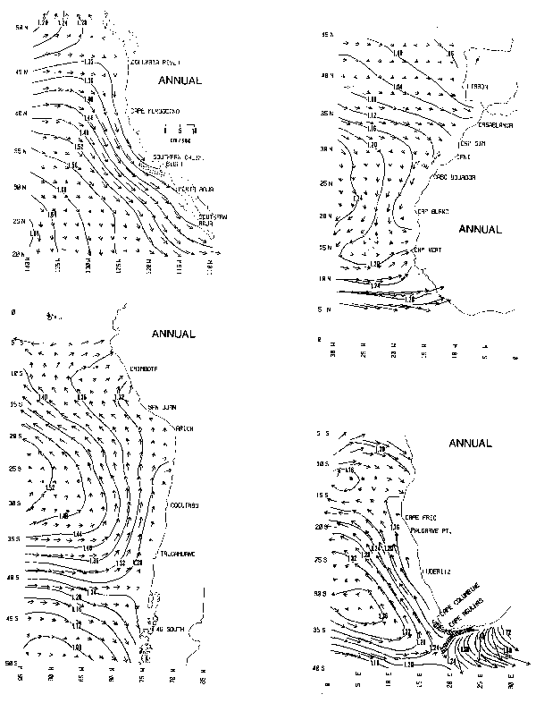
Chart 1. Annual mean surface geostrophic flow (0/1000 db, cm sec-1) and dynamic topography (dyn m).
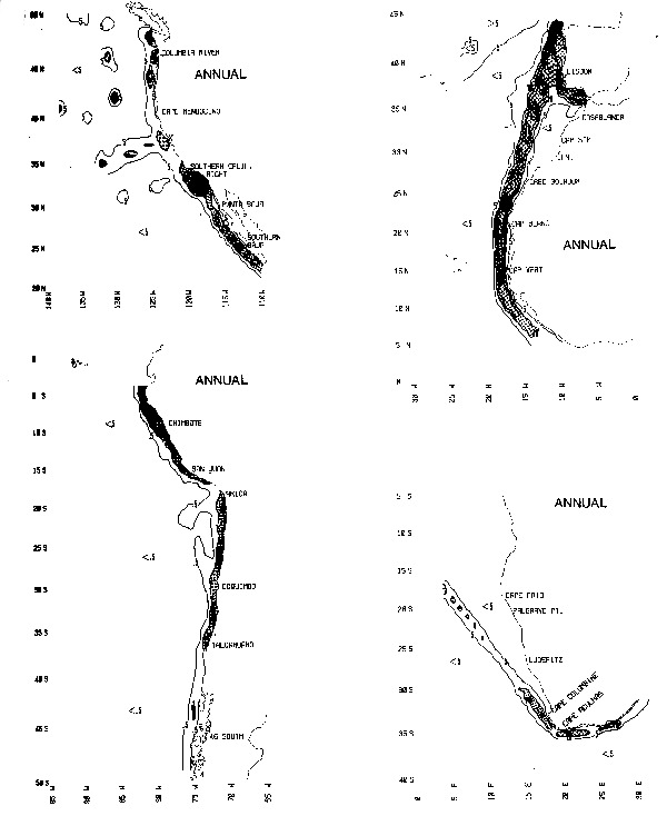
Chart 2. Distributions of observations per 1-degree square (thousands of observations)
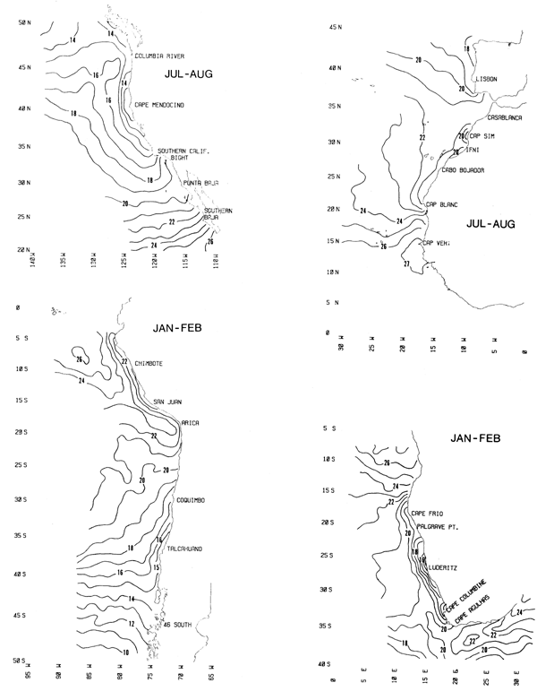
Chart 3. Summer sea surface temperature. (°C)
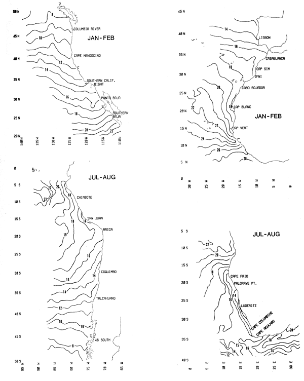
Chart 4. Winter sea surface temperature (°C)
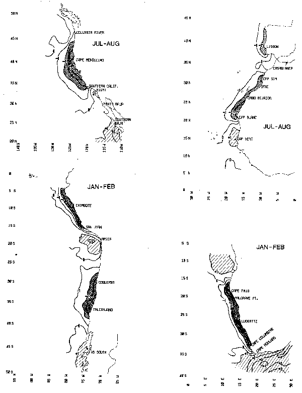
Chart 5. Summer coastal sea surface temperature anomaly (°C)
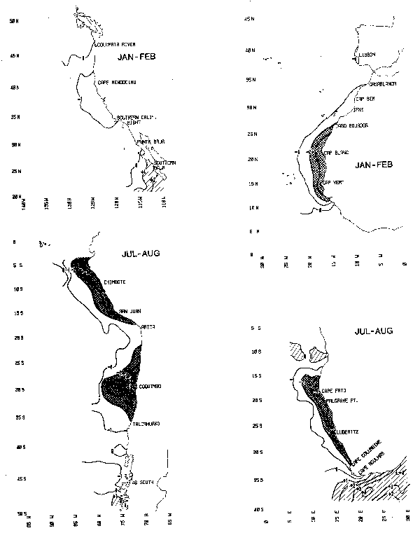
Chart 6. Winter coastal sea surface temperature anomaly (°C)
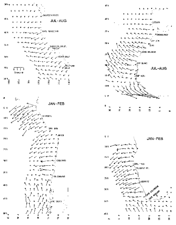
Chart 7. Summer surface Ekman transport (t sec-1m-1)
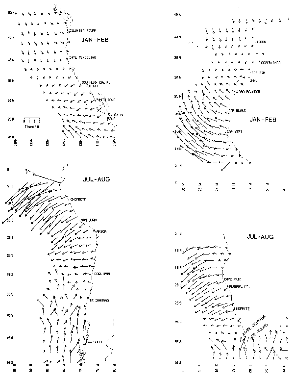
Chart 8. Winter surface Ekman transport (t sec-1m-1)
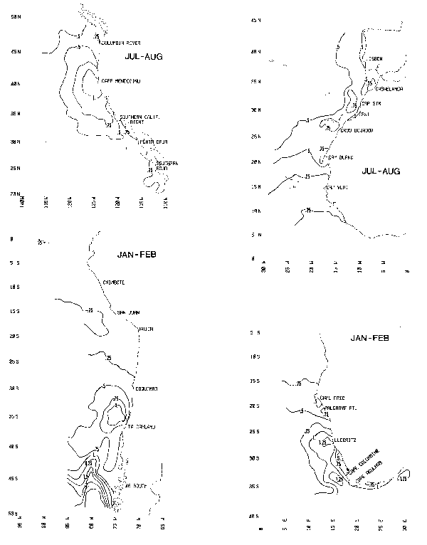
Chart 9. Summer distributions of wind speed cubed (units of 1000 m3sec-3).
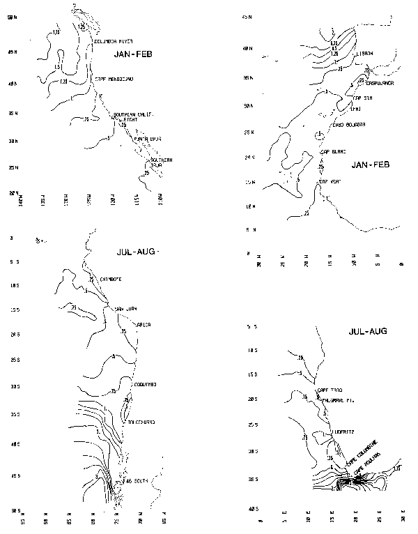
Chart 10. Winter distributions of wind speed cubed (units of 1000 m3sec-3).
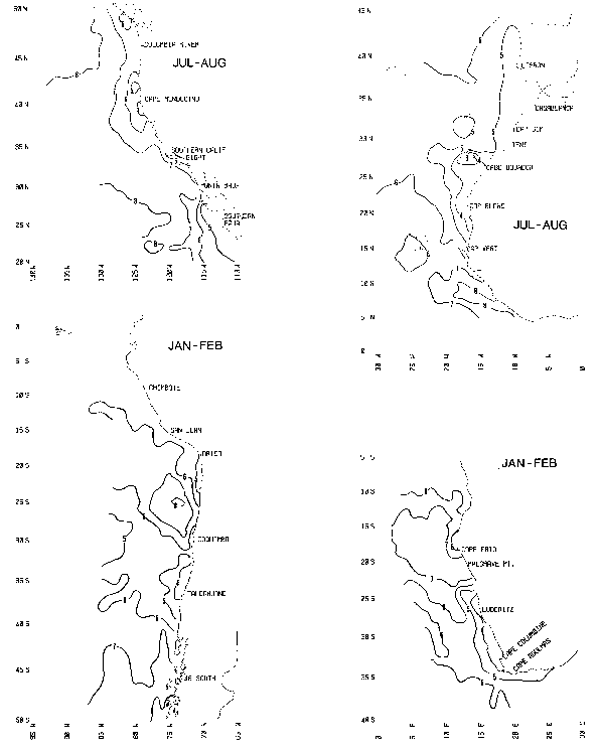
Chart 11. Summer distributions of total cloud amount (tenths of sky obscured).
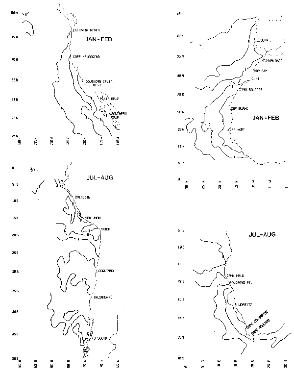
Chart 12. Winter distributions of total cloud amount (tenths of sky obscured).
REFERENCES
Ahlstrom, E.H. 1959. Vertical distribution of pelagic fish eggs and larvae off California and Baja California. U.S. Fish Wildl.Serv., Fish.Bull. 60:107–146.
Ahlstrom, E.H. 1965. Kinds and abundance of fishes in the California Current region based on egg and larval surveys. Calif.Coop.Oceanic Fish.Invest., Rep. 10:31–52.
Badenhorst, A. and A.J. Boyd. 1980. Distributional ecology of the larvae and juveniles of the anchovy Engraulis capensis Gilchrist in relation to the hydrological environment off South West Africa, 1978/79. Fish.Bull.S.Afr. 13:83–106.
Bakun, A. 1973. Costal upwelling indices, west coast of North America, 1946–71. U.S. Dep.Commer. NOAA Tech.Rep.NMFS SSRF- 671, 103 p.
Bakun, A. and C.S. Nelson. 1977. Climatology of upwelling related processes off Baja California. Calif. Coop.Oceanic Fish.Invest.Rep. 19:107–127.
Bakun, A. and R.H. Parrish. 1980. Environmental inputs to fishery population models for eastern boundary current regions. In Workshop on the effects of environmental variation on the survival of larval pelagic fishes, Lima, Peru. 20 April–5 May 1980. IOC Workshop Rep. 28, UNESCO, Paris, p. 67–104
Bakun, A. 1982. Turbulence, transport and pelagic fish in the California and Peru Current systems. Calif.Coop.Oceanic Fish.Invest.Rep. 23:99–112.
Bakun, A., D.R. Mclain and F.V. Mayo. 1974. The mean annual cycle of coastal upwelling off western North America as observed from surface measurements. Fish.Bull., U.S. 72(3):843–844.
Bang, N.D. and W.R.H. Adrews. 1974. Direct current measurements of a shelf-edge frontal jet in the southern Benguela system. J.Mar. Res. 32(3):405–417.
Barkley, R.A. 1968. Oceanographic Atlas of the Pacific Ocean. Univ.of Hawaii Press,Honolulu, 20 p., 156 charts
Belveze, H. and J. Bravo de Laguna. 1980. Les resources halieutiques de l'atlantique centre-est. Deuxieme partie: Les ressources de la cote ouest-africaine entre 24°N et le Detroit de Gibraltar. FAO Doc.Tech.sur les peches, FIRM/T 186.2 (Fr.) 64 p.
Bernstein, R.L., l. Breaker and R. Whritner. 1977. California current eddy Formation: ship, air and satelite results. Science. 195;353–359.
Bohnecke, G. 1936. Temperatur, Salzgehalt und Dichte an der Oberflache des Atlantischen Ozeans. Atlas. “Meteor” Rep. 5. 74 charts.
Bravo de Laguna, J., M.A.R. Fernandez and J.C.Santana. 1976. The Spanish fishery on sardine (Sardina pilchardus Walb.) off west Africa. ICES CM 1977/G:13 Pelagic Fish (Southren ) Committee.
Cańon, J.R. 1978. Distribución de la anchoveta (Engraulis ringens Jenyns) en el norte de Chile en relación a determinadas condiciones oceanográficas. Invest.Pesq.Inst.Fom. Pesq. Santiago Chile. 30, 128 p. (Also available in English: J.R. Cańon, Distribution of anchoveta (Engraulis ringens Jenyns) in northern Chile in relation to selected oceanographic conditions, M.S. thesis, Oregon State University, Corvallis, 1973. 106p.
Cram, D. 1981. Hidden elements in the devleopment and implementation of marine resource conservation policy: The case of the South West Africa/Namibian fisheries. In Resource management and environmental uncertainty. (M.H. Glantz and J.D. Thompson, eds ). John Wiley and sons, New York. p. 137–158.
Crawford, R.J.M. 1980. Seasonal patterns in South Africa's western cape purse-seine fishery. J.Fish.Biol. 16:649–664.
Crawford, R.J.M., P.A. Shelton and L. Hutchings. 1980. Implications of availability, distribution and movements of pilchard sardinops ocellata and anchovy Engraulis capensis for assessment and management of the South African purse-seine fishery. Rapp.P.-v.Reun.Cons.int.Explor.Mer. 177:355–373.
Darbyshire, M. 1966. The surface waters near the coasts of southern Africa. Deep-Sea Res. 13(1):57–81.
Ekman, V.W. 1905. On the influence of the earth's rotation on ocean currents. Ark.Mat.Astron.Fys. 2(11):1–55.
Food and Agriculture Organization of the United Nations. 1978. Report of the ad hoc working group on sardine (Sardina pilchardus Walb.) CECAF/ECAF Series/78/7(En), 35 p.
Guillen, O. 1980. The Peru current system. I: Physical aspects. In Proceedings of the workshop on the phenomenon known as “El Nino”. UNESCO, Paris:185–216. In English and Spanish.
Gunther, G.R. 1936. A report on oceanographical investigations in the Peru Coastal Current. Discovery Rep. 13:17–276.
Hart, T.J. and R.I. Currie. 1960. The Benguela Current. Discovery Rep., 31:123–298.
Hessleberg, T.H. and H.U. Sverdrup. 1915. Die Stabilitatsverhaltnisse des Seewassers bei vertikalen Verschiebungen. Bergens Museums Aarbok 1914–15. No. 15, 16 p.
Hickey, B.M. 1979. The California Current System- hypotheses and facts. Progress in Oceanography, 8(4):191–279.
Husby, D.M. and C.S. Nelson. 1982. Turbulence and vertical stability in the California Current. Calif.Coop.Oceanic Fish.Invest.Rep. 23:113–129.
Hughes, P. and E.D. Barton. 1974. Stratification and water mass structure in the upwelling area off northwest Africa in April/May 1969. Deep-Sea Res., 21:611–628.
Huyer, A. 1976. A comparison of upwelling events in two locations: Oregon and Northwest Africa.J.Mar.Res. 34(4):531–546.
Jordán, R.S. 1980. Biology of the anchoveta: I. Summary of the present knowledge. In Proceedings of the workshop on the phenomenon known as “El Niño”. UNWESCO, Paris: 249–278. In English and Spanish.
King, D.P.F. 1977. Distribution and relative abundance of eggs of South West African pilchard Sardinops ocellata and anchovy Engraulis capensis, 1971/72. Fish.Bull.S.Afr., 9:23–31.
Kramer, D. and J.R. Zweifel. 1970. Growth of anchovy larvae (Engraulis mordax Girard) in the laboratory as influenced by temperature. Calif.Coop.Oceanic Fish.Invest.Rep. 14:84–87.
Lafond, E.C. 1951. Processing oceanographic data. U.S. Navy Hydrographic Office, H.O. Pub. No. 614, Washington, D.C. 114 pp.
Lasker, R. 1964. An experimental study of the effects of temperature on the incubation time, development and growth of Pacific sardine embryos and larvae. Copeia, No. 2:399–405.
Lasker, R. 1978. The relation between oceanographic conditions and larval anchovy food in the California Current: identification of factors leading to recruitment failure. Rapp.P.- v.Reun.Cons.int.Explor.Mer. 173:212–230.
Le Clus, F. 1979. Oocyte development and spawning frequency in the South West African pilchard Sardinops ocellata. Fish.Bull.S.Afr. 12:53–68.
Levitus, S. 1982. Climatological Atlas of the World Ocean. U.S.Dep.Commer., NOAA Prof.Pap. 13. 173 p.
Levitus, S. and A.H. Oort. 1977. Global analysis of oceanographic data. Bull,Amer,Meteor,Soc. 58(12):1270–1284.
McDowell, S.B. 1962. Personal letter to A.J. Liebling. p. 189–202. In A.J. Likebling, “Onward and upward with the arts: The soul of bouillabaisse”. The New Yorker, October 27, 1962.
Mittelstaedt, E. 1974. Some aspects of the circulation in the north-west African upwelling area off Cap Blanc. Tethys, 6(1–2):89–92.
Mooers, C.N.K. and J.S. Allen. 1973. Final report of the Coastal Upwelling Ecosystems Analysis Summer 1973. Teoretical Workshop. School of Oceanography, Oregon State Univ. Corvallis, Oregon. 212 p.
Nelson, C.C. 1977. Wind stress and wind stress curl over the California Current. U.S. Dep.Commer. NOAA Tech.Rep. NMFS SSRF-714, 87 p.
Nelson, C.S. and D.M. Husby. 1983. Climatology of surface heat fluxes over the California Current region. U.S.Dep.Commer. NOAA Tech.Rep. NMFS SSRF-763, 155 p.
Nelson, G. and L. Hutchings. MS. The Benguela upwelling area. Sea Fisheries Institute, Cape Town, South Africa, 32 p.
Neumann, G. and W.J. Pierson, Jr. 1966. Principles of Physical Oceanography, Prentice-Hall, Englewood Cliffs, 545 p.
Niller, P.P. and E.B. Kraus. 1977. One-dimensinal models of the upper ocean. p. 143–172. In Modelling and prediction of the upper layers of the ocean. (E.B. Kraus, ed.) Pergamon Press, New York,
Parrish, R.H., C.S. Nelson and A. Bakun. 1981. Transport mechanisms and reproductive success of fishes in the California Current. Biol. Oceanogr. 1(2):175–203.
Pauly, D. 1981. The relationships between gill surface area and growth performance in fish: a generalization of von Bertalanffy's theory of growth. Meeresforschung. 28:251–282.
Pavlova, Y.V. 1966. Seasonal vartiations of the California Current. Oceanol. 6(6):806–814.
Radovich, J. 1981. The collapse of the California sardine fishery: what have we learned? p. 107– 306. In Resource management and enviornmental uncertainy: lessons from coastal upwelling fisheries. (M.H. Glantz and J.D. Thopson, eds.) John Wiley and Sons, New York,
Rebert, J.P. 1978. Note on the hydrology of the west African continental shelf, from mauritania to Guinea (Annex 9). p. 87–92. In Report of the ad hoc working group on West African coastal pleagic fish from Mauritania to Liberia (26oN to 5oN). CECAF/ECAF Series 78/10 (En).
Reed, R.K. and D. halpern. 1976. Observations of the California Undercurrent off Washington and Vancouver island. Limnol.Oceanogr. 21(3):389–398.
Reid, J.L., Jr. 1967. Oceanic environments of the genus Engraulis around the world. Calif.Coop.Oceanic Fish.Invest. Rep. 11;29–33.
Reid, J.L., Jr., G.I. Roden and J.G. Wyllie. 1958. Studies of the California Current System. Calif.Coop.Oceanic Fish.Invest.,Prog.Rep., 1 July 1956 to 1 January 1958. p. 27.57
Robles. F.L.E. 1979. Water masses and circulation in the S.E. Pacific and the “El Nino” event, Ph.D. Thesis, University of Wales, Swansea, 175 p. 156 charts.
Santander, H. and O.S. de Castillo. 1979. El inctioplantion de la Coata Peruana. Bol.Inst.Mar.Puru. 4(3):69–112.
Serra, J.B., M.H. Aguayo, O.J. Rojas, F.C. Inostroza and J.C. Cannon, Sardina Española. 37 p. In Estado actual de principales pesquerias nacionaloes. Instituto de Fromento Pesquero, Chile, Shannon, L.V. 1970. Oceanic circulation off South Africa. Fish.Bull.S.Afr. 6:27–33.
Shelton, P.A. and L.Hutchings. 1982. Transport of anchovy, Engraulis capensis Gilchirst, eggs and early larvae by a frontal jet current. J.Cons.int.Explor.Mer. 40:185–198.
Silva. S.N. and S. Neshyba. 1979. On the southernmost extension of the Peru-Chile Undercurrent. Deep-sea Res. 26A:1387–1393.
Smith, R.L. 1978. Physical oceanography of coastal upwelling regions. A comparison: Northwest Africa, Oregon and Peru. Symposium on the Canary Current. Upwelling and Living Resources, No. 40, 10 p.
Stander, G.H. 1964. The pilchard of South West Africa. The Benguela Current off South West Africa. Investl.Rep.Mar.Res.Lab., S.W.Afr. 12, 122 p.
Stander, G.H. and A.H.B. de Decker. 1969. Some physical and biological aspects of an oceanographic anomaly off South West Africa in 1963. Investl.Rep.Div.Sea Fish.S.Afr. 81:1–46.
Sverdrup, H.U. and R.H. Fleming. 1941. The waters off the coast of Southern California, March to July 1937. Bull.Scrips Inst.Oceanogr. Univ. of Calif. La Jolla. 4:261–378.
Sverdrup, H.U., M.W. Johnson and R.H. Fleming. 1942. The oceans: their physics, chemistry and general biology. Prentice-Hall, Englewood Cliffs. 1087 p.
Iomezak, M., jr. 1981. Prediction of environmental changes and the struggle of the third world for national independence: The case of the Peruvian fisheries. p. 401–438. In Resource management and environmental uncertainty. (M.H. Glantz and J.D. Thompson, eds.) John Wiley and Sons, New York.
Iroadec, J.-P., W.G. Clark and J.A. Gulland. 1980. A review of some pelagic fish stocks in other areas. Rapp.P.-v.Reun.Cons.int.Explor.Mer. 177:252–277.
Wooster, W.S. and J.H. Jones. 1970. California undercurrent off northern Baja California. J.Mar.Res. 28(2):235–250.
Wooster, W.S. and J.L. Reid, Jr. 1963. Eastern boundary currents. p. 253–280. In The Sea. Vol. 2. (M.N. Hill, ed.) Interscience Publ., New York.
Wooster, W.S. and H.A. Sievers. 1970. Seasonal variations of temperature, drift, and heat exchange in surface waters off the west coast of South America. Limnol.Oceanogr. 15:595–605.
Wylie, J.G. 1966. Geostrophic flow of the California Current at the surface and at 200 m. Calif.Coop.Oceanic Fish.Invest.,Atlas No.4, XXII p, 288 charts.
Wyrtki, K. 1965. Summary of the physical oceanography of the eastern Pacific Ocean. Inst. of Mar.Res.Ref. 65–10, Scripps Inst.Oceanogr., Univ. of Calif., La Jolla. 69 p. 9 charts.
by
John J. Magnuson1 and Larry B. Crowder2
1Center for Limnology and
Department of Zoology
University of Wisconsin
USA
2Department of Zoology
North Carolina State University
Raleigh, North Carolina 27605
USA
Resumen
Las comunidades de peces planctivoros del Lago Michigan han fluctuado grandemente tanto en la composición por especies como en abundancia. La pesquería ha variado drámaitcamente durante el ultimo siglo. Granparte de la variabilidad ha ocurrido a través de disturbios no intencionados y manipulaciones planedas por el hombre.
Los estudios descritos se centran en la alosa (Alosa psuedoharangus), eper- lano arco iris (Osmerus mordar), y juveniles de arenque (Coregonus hoyi). La alosa y el eperlano arco iris son peces exóticos mientras que el arenque es una especie sobreviviente de aguas profundas del lago.
La Lamprea de Mar invadió el sistema de los Grandes Lagos en 1829 y junto con las pesquerías selectivas por tamanos, eliminaron especies de peces comerciales de tamaño grande a mediados de los años 1950s. El eperlano entró al sistema en 1912, aumentando rápidamente en el Lago Michigan a mediados de los años 1930s. La aIosa invadió el sistema y aumento dramaticamenteo los años 1960s. Entre los planetívoros nativos se incluyen siete especies de Coregonus de las cuales seis se han extinguido desde que el aumento de alosa comenzo.
El Lago Michigan es un sistema relativamente grande pero de baja diversidad, es también un sistema relativamente cerrado, y por lo tanto tiene una pobre amortiguación contra los cambios.
Se ha documentado la competencia entre alosa, eperlano y peces planetívoros nativos, aparentemente la fuerte competencia entre alosa y arenque ha resultado en cambios en las características del aparato alimenticio del arenque desde los años 1960s. También se han documentado cambios ecológicos, y el arenque ha desplazado a la alosa después que estos cambios ocurrieron. Se revisa la compleja evolución de estas interacciones y se considera que la competencia es una fuerza causal importante de los cambios observados en las comunidades.
Ciertamente la predacíon es una causa importante de los cambios inducidos por la Lamprea de Mar. También la predación de huevos por parte de los peces exóticos ha sido clave en la reducción de especies planetívoras nativas. Se discuten las fluctuaciones del reclutamiento inducidas por predación de huevos así como los posibles efectos de la reintrodución de algunas especies que han estaido ausentes del Lago Michigan por algún tiempo.
Estas observaciones están relacionadas con los sistemas océanicos neríticos y sus cambios.
INTRODUCTION
Competition and predation are two species interactions that are important in the dynamics of fish assemblage structure. The planktivorous fish assemblages of Lake Michigan (North America) have fluctuated greatly both in species composition and in the abundance of individual species. Our purpose here is to evaluate the evidence for the importance of competition and predation in these dynamics. We also consider the applicability of results from Lake Michigan to other neritic systems.
The fish communities and thus the fisheries of the Laurentian Great Lakes of North America have been highly variable over the past half century. This variability has complicated the use and management of the fishery resources. Much of this variability (population extinctions, exponential growth of exotic fishes, the collapse and reopening or genesis of commercial and sport fisheries) has occurred through unintentional disturbances and planned manipulations by humans. These large-scale variations are best known in Lake Michigan (Smith 1970; Wells and McLain 1972, 1973; Christie 1974) and serve as experiments on fish community structure and species interactions in a low diversity, neritic fishery.
Our attention focuses on the three abundant pelagic planktivores -- the alewife Alosa pseudoharengus, the rainbow smelt Osmerus mordar and the young of bloaters Coregonus hoyi. The alewife and smelt are exotics and the bloater is a surviving species of deep water lake herring or cisco. The dynamics of these three species were greatly influenced by the interactions between the sea lamprey Petromyzon marinus and the primary native piscivore - lake trout Salvelinus namaycush (Lawrie 1970). The sea lamprey invaded the Upper Great Lakes via the Welland Canal built around Niagara Falls in 1829. Together with a size selective fishery, sea lamprey eliminated the larger commercial fishes including lake trout by the mid 1950s. Smelt was introduced into the Lake Michigan drainage in 1912 and subsequently spread throughout the Upper Great Lakes, increasing rapidly in Lake Michigan in the 1930s. Alewife invaded the Great Lakes via the Welland Canal and increased exponentially in the early 1960s, presumably due to the absence of large piscivores. Native planktivores originally included 7 native ciscoes. Six of these went extinct during the increase of alewife and rainbow smelt.
By the mid 1960s Lake Michigan was yielding little of its natural productivity to commercial or sport fisheries. In response to this problem management measures were taken to reduce sea lamprey populations with a selective toxicant for ammocetes (Lawrie 1970). Then lake trout and several non-native piscivores were restocked, beginning in 1965. The salmonid stocking program in Lake Michigan has led to a valuable sport fishery. However, natural reproduction of stocked salmonids is still relatively rare. Thus the system depends strongly on fishery management to stock piscivores and control sea lamprey.
We think that an understanding of predation and competition among the planktivores is important to fishery management decisions for Lake Michigan. The effects of these processes apparently have contributed greatly to the instability of the fisheries in Lake Michigan. In addition, the three planktivores abundant now (alewife, smelt, and bloater) provide both the forage base for the salmonid sport fishery and in the case of the bloater an important commercial fishery.
A number of characteristics of Lake Michigan make it useful for examining the importance of species interactions in neritic fisheries. First, the extent of historical manipulations and their documentation is perhaps unparalleled. Second, recent laboratory and field observations on resource use, foraging behavior and functional morphology provide clues for interpreting historical as well as contemporary data. Third, Lake Michigan while moderately large (1/10 the area of the North Sea) is a relatively closed system. This reduces colonization from other stocks of the same species or from other species with similar characteristics. Fourth, Lake Michigan is a low diversity system relative to many nearshore marine systems. These last two characteristics suggest that the Lake Michigan fish community may be more poorly buffered and less resilient to change than nearshore marine fish communities. This poor buffering may allow the effects of species interactions among planktivores in Lake Michigan to be more easily observed than in comparable marine systems.
COMPETITION
Alewife, smelt and native planktivores use the same food resources. Both native and exotic planktivores in Lake Michigan shared many prey types (Wells and Beeton, 1963; Morsell and Norden, 1968; Janssen and Brandt 1980; Wells 1980; Crowder et al .,1981). Also large- bodied zooplankton may have become limiting during the increase of alewife (Wells 1960, 1970). A dramatic reduction in the mean size of zooplankton at the peak of alewife abundance suggests intense planktivory and limited food resources of preferred size for planktivores. This absence of large-bodied zooplankton may have favored alewife over the native ciscoes.
Available data on the feeding behavior of alewife and the bloater support the idea that alewife is more efficient at feeding on small prey owing to ability to switch feeding modes from particulate feeding to filtering (Janssen 1976; Crowder and Binkowski 1983). But bloater appears to be more efficient than alewife when foraging on benthic prey. The zooplankton feeding stage, in bloater then becomes a “bottleneck” for recruitment of larger bloaters to the benthos. If bloaters make it through the zooplankton feeding stage, it appears that they can succeed relative to alewife in the near bottom habitat.
Alewife and smelt may compete for food. Smelt and alewife eat similar foods (Crowder et al., 1981) and smelt decreased in abundance as alewife increased in abundance in Lake Michigan (Christie, 1974).
Competition for food among the species may be minimized by spatial segregation of competitors. Temperature drives physiological rates and thus has important consequences for survival and growth of fishes (Kitchell et al., 1977). In pelagic systems, temperature may provide a gradient for spatial segregation of species with similar food habits (Magnuson et al., 1979). Brandt et al. (1980) provided evidence for segregation by thermal habitat of major planktivores in Lake Michigan. Complementarity in the use of thermal habitat and food has also been demonstrated in Lake Michigan fishes (Crowder et al., 1981). Native fishes that overlap the thermal habitats of alewife and smelt use different foods. This pattern of resource subdivision often has been attributed to competition (Schoener 1974), though other interactions and environmental changes will certainly influence resource use.
Additional lines of evidence for competition between alewife and bloater deal with the habitat and diet shifts of bloater and character displacements of the feeding apparatus of bloater that occurred when alewife became abundant. During this period, young bloater shifted to a more benthic life style and had a reduction in the length and number of gill rakers (Crowder MS, b).
Prior to the increase of alewives, bloaters less than 178 mm were rarely caught in extensive bottom trawling over several years (Wells and Beeton 1963; Wells 1968). A few bloaters less than 178 mm were caught in midwater trawls and these were primarily zoo- planktivorous (Wells and Beeton, 1963). Small bloaters (49–145 mm) are now caught regularly on the bottom (Crowder and Magnuson, 1982). Of the fishes caught in 48 tows during August 1979, 42% were bloaters, 71% of which were small-sized individuals. These small bloaters were probably young-of-year and yearlings based on their size (Edward Brown, Jr., Great Lakes Fishery Laboratory, U.S. Fish and Wildlife Service, Ann Arbor, Michigan). Diets of these small bloaters were dominated by benthic prey, especially the large amphipod Pontoporeia hoyi, (Crowder MS, a). Bloaters collected in 1979 also have significantly fewer and shorter gill rakers than those collected in 1960 by Stan Smith (Great Lakes Fishery Laboratory, U.S. Fish and Wildlife Service, Ann Arbor, Michigan, unpublished data) (Crowder MS, b). Both ecological and morphological data suggest an earlier shift to benthos in bloaters following the alewife invasion. These habitat, diet, and morphological changes are striking and would reduce competition with the more efficient pelagic planktivore, the alewife.
This evolving difference in life style of bloater in the face of competition with alewife for zooplankton may also explain another habitat shift we observed as bloater increased in abundance during the later 1970s (Crowder and Magnuson, 1982). But in this case the bloater in the near bottom waters displaced the alewife. When we began our study of species interactions in Lake Michigan in 1977, bloaters were extremely rare. The commercial fishery for bloaters had been closed and our catch of bloaters in fall 1977 amounted to 0.3% of the total fish caught in all day bottom trawls. Alewife were abundant in all day bottom trawling and occurred at temperatures preferred in the laboratory. We repeated the 1977 sampling in fall 1979. Between 1977 and 1979, bloater occupied the thermal habitat that had been occupied by alewife in 1977 and adult alewife near bottom at night occupied colder water (Crowder and Magnuson, 1982). Bloater appears more efficient than alewife when feeding on near bottom food resources (Crowder and Binkowski, 1983). Since total catch of alewife was not reduced in 1979, and since predation intensity by salmonids on alewife did not change drastically between 1977 and 1979 (Stewart et al. 1981), we favor the hypothesis that the altered thermal distribution of alewife resulted from competitive interactions with bloater (Crowder and Magnuson, 1982).
These later observations (i.e., bloater wins) also suggest that the interaction leading to the initial declines of native ciscoes including bloater was more complex than the simple competitive advantage of alewife. The ability to filter smaller zooplankton confers a competitive advantage on alewife when small zooplankton predominate as they did in the mid 1960s in Lake Michigan. If zooplankton are large, as they are now (Gitter, 1982) bloater young-of-year do not suffer this relative disadvantage (Crowder and Binkowski 1983). Following the reintroduction of piscivores into Lake Michigan, forage fish populations (especially alewife) were reduced and zooplankton increased in size relative to those observed at the peak of alewife abundance. It appears then that bloaters now recruit well through the zooplankton feeding stage, given reduction in alewife abundance induced by introduced piscivores - the salmonids and lake trout.
We conclude that competition has been an important interaction among Lake Michigan planktivores. Competition among adult fishes likely regulates resource use. Competition among fishes in the first year or so of life may contribute to the inverse changes in the abundances of these species - namely the declines of native ciscoes as smelt or more importantly alewife increased in abundance.
PREDATION
Predation is well documented as an important contributor to at least one species extinction in Lake Michigan. The sea lamprey played a dominant role in the extinction of lake trout (Wells and McLain, 1972, 1973). The expanding populations of exotic alewife and smelt are implicated as a cause of observed extinctions and massive population declines of many fishes in Lake Michigan. Although competition for food resources as discussed above has been the most commonly proposed mechanism for these interactions, predation on fish eggs and ichthyoplankton also has been implicated as a mechanism as well (Crowder, 1980). Predation on fish eggs and larvae by alewife and smelt should be evaluated as a possible influence on year-to-year differences in the recruitment of native fishes that still persist, such as the bloater.
We suggest that the probability that a predator-caused extinction is more probable if the predator (1) has recently increased in abundance, (2) has a large population biomass and thus a high population consumption rate, (3) has a preference for the size or taxon in question but can maintain a high abundance on alternate prey and (4) has recruitment that is relatively independent of that prey organism's abundance. These characteristics apply to the sea lamprey, and possibly to the alewife and the smelt.
The sea lamprey increased greatly in abundance after its invasion (Shetter, 1949). Its preferred prey was lake trout (Smith, 1968). As the lake trout declined in abundance, scarring from lamprey feeding activity increased on lake whitefish Coregonus clupeaformis, common suckers Catostomus commersoni, and other species (Shetter, 1949). The abundance of sea lamprey remained high as lake trout went extinct and lamprey control measure did not become effective in Lake Michigan until after the extinction of lake trout (Wells and McLain, 1972, 1973). Also the sea lamprey spawns in streams and its young live in the soft sediments as detritivores for several years, safe from any predation by lake trout. When they metamorphose to the parasitic form and return to the lake they are already predators on the lake trout. Thus the sea lamprey, as a predator on lake trout, had the characteristics to cause the observed extinction.
The alewife also increased dramatically in abundance after its invasion into Lake Michigan (Smith 1968; Wells and McLain, 1972, 1973). Although it can feed efficiently on smaller zooplankton, i.e. it has alternate prey (Janssen,1976; Crowder and Binkowski, 1983), its feeding preference is for zooplankton forms (Brooks and Dodson, 1965; Brooks, 1968). It was during this period of maximum alewife abundance that the mean size of zooplankton was reduced (Wells 1970). Pelagic fish eggs and ichthyoplankton were similar in size to the larger crustacean zooplankton that were reduced (Crowder 1980). Could predation by alewife on pelagic fish eggs and larvae have caused the many extinctions that occurred among native planktivores at that time of maximum alewife abundance?
Some circumstantial evidence exists for the idea that predation by plantivores on pelagic fish eggs and larvae contributed to the decline of native species (Crowder 1980). Pelagic eggs and larvae should be more available than demersal ones to pelagic planktivores such as smelt and alewife. Those species with pelagic eggs and larvae should have been more affected by alewife and smelt than were species with benthic eggs or larvae. Of the 21 species common prior to the invasions, 10 or about half had pelagic eggs, based on Balon's (1975) classification of reproductive guilds. After the increase of alewife (and smelt), only two of these species remained abundant. Eight are either extinct or rare. None of those with benthic eggs or larvae went extinct. A comparison between one pair of congeners makes the difference even more clear. Emerald shiner Notropis athorenoides with large pelagic eggs was abundant until about 1960 in southern Lake Michigan, and had supported a minor bait fishery. It was extinct by 1963 when alewife was abundant (Smith 1970). The congener, the spottail shiner Notropis hudsonius, with small demersal eggs did not become extinct (Crowder 1980).
As zooplankton were reduced by alewife in the 1960s, zooplankters, longer than 1.1 mm became extremely rare (Wells 1970). The eggs and early larvae of the 10 fishes with pelagic eggs should have become rare provided alewife responded to them in the same way as they did to larger zooplankton. The diameters of these eggs ranged from 1.25 to 3.25 mm (see Crowder 1980) or the sizes on which alewife would be more likely to gulp or particulate feed than to filter feed (see Crowder MS, a). These eggs and their larvae are certainly large enough and energetically profitable enough to be selected by planktivores. Alewife in lakes eat fish eggs (Morsell and Norden 1968) and fish larvae (Kohler and Ney 1980). The fish larvae were 9 to 26 mm long. Kohler and Ney (1980) suggested that their piscivory may have contributed to the collapse of Great Lakes fishes. However, no laboratory data exist on the selection of eggs or larvae from a pool of smaller zooplankton which are several orders of magnitude more abundant.
Alewife eggs, larvae and young tend to be in waters less than 5 m deep and thus would be largely free of predation both by the deep water ciscoes that went extinct and the surviving bloater.
We think that the alewife has the characteristics to cause an extinction of fishes with pelagic eggs and larvae in Lake Michigan with predation as the mechanism. Experiments on selective feeding on eggs and larvae are needed to confirm this inference.
Smelt has some of the same characteristics but they are less well documented. Also alewife may have influenced the abundance of smelt.
The next question is whether year-to-year variations in alewife in Lake Michigan can cause year-to-year fluctuations in the recruitment of fishes with pelagic eggs and larvae. Alewife are less abundant now than in the 1960s owing to predation on them by stocked salmonids (Stewart et al. 1981). As expected, the mean size of zooplankton has increased since the time of maximum alewife abundance (Wells 1970; Gitter 1982) presumably from the lowered rate of predation by alewife on zooplankton. The abundance of adult alewife now fluctuates from year-to-year by a factor of two or so (Hatch et al 1981) and the species composition and mean size of the zooplankton vary from year to year (Gitter 1982). Thus, there is some evidence that zooplankton are responding to fluctuations in alewife abundance. Also bloaters are again producing strong year classes and one could speculate that reduced predation on eggs and larvae have contributed to this. Hunter (1982) argued for the role of predation in the recruitment process of marine fish. And John Hunter and John Magnuson hypothesized in Fish Ecology III (Rothschild and Rooth 1982) that planktivores as selective egg and larval predators could significantly influence year-to- year variations in recruitment of fishes via predation on planktonic eggs and larvae.
The alewife and perhaps the smelt in Lake Michigan appear to meet the necessary criteria. They are abundant, vary in abundance from year to year, and feed selectively on larger zooplankton. However, there is no direct evidence that they select the eggs and larvae from a pool of more abundant but small zooplankton. The hypothesis should be tested in a pelagic ecosystem. Lake Michigan may be an ideal model for the test because species diversity of the planktivore assemblage is low, a reasonable base of biological information is available on the taxa involved, and few invertebrate predators are there to complicate the study.
The next event in which predation may play a role in Lake Michigan is for stocked salmonid piscivores to alter the relative abundance of the three dominant planktivores-the alewife, smelt and bloater (Stewart et al. 1981). Stocking rates of salmonid are regulated by fishery management and may not track changes in the abundance of alewife, their dominant prey. Major time lags occur between a decision to stock and when the impact on the forage base occurs (Stewart et al. 1981). This “predator inertia” is at least 3 years for coho Oncorhynchus kisutch and chinook O. tshawytscha salmon and 5 or 6 years for lake trout (Stewart et al. 1981). Since alewife abundance has peaked about every 4 years during the late 1960s and early 1970s, salmonid stocking cannot be used as a tool to moderate these short-term variations. The problem is further complicated because of time lags involved in the assessment of alewife populations. Stocking rates therefore are set for some average condition and the potential for a mismatch between the abundance of salmonids and their prey, the alewife, is quite high in some years. Year class failures of the alewife and a shift of the salmonids to alternate prey are the expected consequences.
Our conclusions about the influence of predation on the dynamics of the assemblage of planktivores in Lake Michigan are not as firm as were our conclusions about competition. This is surprising to us since the influence of predation has generally been believed to be easier to demonstrate than the effects of competition (Connell 1975; MacLean and Magnuson 1977; Sale 1979). We do conclude that predation on pelagic eggs and larvae by alewife and smelt is implicated as a cause of extinction of fishes with pelagic eggs and larvae. Predation also may contribute to year-to-year variation in the recruitment of the surviving native planktivores such as the bloater. Predation on alewife by stocked salmonids should decrease any influence of alewife on fishes with planktonic eggs and larvae but also may cause occasional year class failures in the alewife.
APPLICABILITY TO LARGER NERITIC ECOSYSTEMS
Lake Michigan is large enough for researchers to feel that the scales on which they are working are oceanic. Yet, the role of scale on the effects of predation and competition in small isolated lakes, the Great Lakes of Africa and North America, and the expanse of the world's major seas and oceans, is poorly known. If the species interactions (competition and predation) among pelagic planktivores in lakes are greatly influenced by the “island” nature of lakes, how are the interactions of pelagic planktivores in ocean systems influenced by the “continental” nature of oceans? On what dimensions should the gradients among these aquatic environments be scaled to account for any differences in the effects of competition and predation?
In Lake Michigan the assemblage of pelagic planktivores excluding ichthyoplankton differs from larger neritic systems in at least two ways important to this paper. First, Lake Michigan is more closed to immigration species (3 planktivores at present in Lake Michigan) and is lower than our perception of species richness for many oceanic systems.
The closed or “island”-like nature of lakes is linked to their sensitivity to the invasion of predators that evolved in other systems (Magnuson 1976). The sea lamprey, the alewife, and the smelt are examples from Lake Michigan, Also in a more closed system interactions with new species are more likely to continue to extinction and to an altered community structure (both taxonomically and functionally). We expect this because immigration of new taxa or individuals is less likely to perturb the processes in a closed system than in a more open system. In an open system, recolonization could follow more closely a local extinction than in a closed system.
Species richness or diversity has often been associated with ecosystem stability in the ecological literature. Certainly in a more species-rich system, substitutions by similar species would be more probable than in a system with only a few species. Thus, the consequences of fluctuations in the abundance of a species may be greater in a species- poor system than in a species-rich system.
Among pelagic planktivores excluding ichthyoplankton, our perception is that ocean systems may be more diverse and are certainly more open than lake systems. We think these factors should have some influence on the effects of species interactions on the dynamics of these fish assemblages. More importantly, these factors plus the smaller size of Lake Michigan may make it easier to observe the effects of species interactions in Lake Michigan than in marine systems. This does not preclude the importance of these interactions in marine systems but suggests that Lake Michigan may be a useful model for observing the potential effects of predation and competition in neritic marine systems.
ACKNOWLEDGEMENTS
We thank T. Frost, C. Paszkowski and W. Tonn for critically reviewing an earlier draft.
REFERENCES
Balon, E.K. 1975. Reproductive guilds of fishes: a proposal and definition. J.Fish.Res.Board Can. 32:821–864.
Brandt, S.B., J.J. Magnuson and L.B. Crowder. 1980. Thermal habitat partitioning by fishes in Lake Michigan. Can.J.Fish.Aquat.Sci. 37:1557–1564.
Brooks, J.L. 1968. The effects of prey size selection by lake planktivores. Syst.Zool. 17:273–291.
Brooks, J.L. and S.I. Dodson. 1965. Predation, body size, and the composition of plankton. Science . 150:28–35.
Connell, J.H. 1975. Some mechanisms producing structured natural communities: a model and evidence from field experiments. In Ecology and Evolution of Communities. (M.L. Cody and J.M. Diamond, eds). Belknap Press, Harvard University Press, Cambridge, Massachusetts.
Crowder, L.B. 1980. Alewife, rainbow smelt and native fishes in Lake Michigan: competition or predation? Env.Biol.Fish. 5:225–533.
Crowder, L.B. MSa. Optimal foraging and feeding mode shifts in fishes.
Crowder, L.B. MSb. Competition and character displacement in a native cisco in Lake Michigan: morphological and ecological evidence.
Crowder, L.B. and F.P. Binkowski. 1983. Foraging behaviors and the interaction of alewife (Alosa pseudoharengus) and bloater (Coregonus hoyi). Envir.Biol.Fish. In press.
Crowder, L.B. and J.J. Magnuson. 1982. Thermal habitat shifts by fishes at the thermocline in Lake Michigan. Can.J.Fish.Aquat.Sci. 39:1046.
Crowder, L.B., J.J. Magnuson and S.B. Brandt. 1981. Complementarity in the use of food and thermal habitat by Lake Michigan fishes. Can.J.Fish.Aquat.Sci. 38:662–668.
Christie, W.J. 1974. Changes in fish species composition of the Great Lakes, J.Fish.Res.Board Can. 31:827–854.
Gitter, M.J. 1982. Thermal distribution and community structure of Lake Michigan zooplankton with emphasis on the interactions of young-of-year fishes. MS Thesis. (Oceanography and Limnology) University of Wisconsin, Madison.
Hatch, R.W., P.M. Haack and E.H. Brown, Jr. 1981. Estimation of alewife biomass in Lake Michigan, 1967–1978. Trans.Am.Fish.Soc. 110:575–584.
Hunter, J.R. 1982. Predation and recruitment. In Fish Ecology III – A Foundation for REX Recruitment Experiment (B.J. Rothschild and C.G.H. Rooth, eds). University of Miami Technical Report 82008
Janssen, J. 1976. Feeding modes and prey size selection in the alewife (Alosa pseudoharengus). J.Fish.Res.Board Can. 33:1972–1975.
Janssen, J. and S.B. Brandt. 1980. Feeding ecology and vertical migration of adult alewife (Alosa pseudoharengus) in Lake Michigan. Can.J.Fish.Aquat.Sci. 37:177–184.
Kitchell, J.F., D.J. Steward and D. Weininger. 1977. Applications of a bioenergetics model to yellow perch (Perca flavescens) and walleye (Stizostedion vitreum vitreum). J.Fish.Res.Board Can. 34:1922–1935.
Kohler, C.C. and J.J. Ney. 1980. Piscivority in a land-locked alewife (Alosa pseudoharengus) population. Can.J.Fish.Aquat.Sci. 37:1314–1317.
Lawrie, A.H. 1970. The sea lamprey in the Great Lakes. Trans.Am.Fish.Soc. 99:766–775.
MacLean, J.H. and J.J. Magnuson. 1977. Inferences on species interactions in percid communities. J.Fish.REs.Board Can. 34:1941–1945.
Magnuson, J.J. 1976. Managing with exotics — a game of chance. Trans.Am.Fish.Soc. 105(1):1–9
Magnusson, J.J., L.B. Crowder and P.A. Medvick. 1979. Temperature as an ecological resource. Am.Zool.. 19:331–343.
Morsell, J.W. and C.R. Norden. 1968. Food habits of the alewife, Alosa pseudoharengus, in Lake Michigan. Proc.Conf.Great Lakes Res. 11:96–102
Rothschild, B.J. and C.G.H. Rooth. 1982. Fish Ecology III — A Foundation for REX a Recruitment Experiment. University of Miami Technical Report 82008.
Sale, P. 1979. Habitat partitioning and competition in fish communities. In Predator-Prey Systems in Fisheries Management (H.Clepper,ed.). Sport Fishing Institute of Washington, D.C.
Schoener, T.W. 1974. Resource partitioning in ecological communities. Science. 185:27–39.
Shetter, D.S. 1949. A brief history of the sea lamprey problem in Michigan waters. Trans.Am.Fish.Soc. 76:160–176.
Smith, S.H. 1968. Species succession and fishery exploitation in the Great Lakes. J.Fish.Res.Board Can. 25:667–693.
Smith, S.H. 1970. Species interactions of the alewife in the Great Lakes. Trans.Am.Fish.Soc. 99:754–765.
Stewart, D.J., J.F. Kitchell and L.B. Crowder. 1981. Forage fishes and their salmonid predators in Lake Michigan. Trans.Am.Fish.Soc. 110:751–763.
Wells, L. 1960. Seasonal abundance and vertical movements of planktonic crustacea in Lake Michigan. U.S.Fish and Wildl.Serv.Fish.Bull. 60:343–369.
Wells, L. 1968. Seasonal depth distribution of fish in southern Lake Michigan. Fish.Bull.U.S. 67:1–15.
Wells, L. 1970. Effects of alewife predation on zooplankton populations in Lake Michigan. Limnol.Oceanogr. 14:556–565.
Wells, L. 1980. Food of alewives, yellow perch, spottail shiners, trout-perch and slimy and fourhorn sculpins in southeastern Lake Michigan. U.S.Fish and Wildl.Serv.Tech.Papers 98.
Wells, L. and A.M. Beeton. 1963. Food of the bloater, Coregonus hoyi, in Lake Michigan. Trans.Am.Fish.Soc. 92:245–255.
Wells, L. and A.L. McLain. 1972. Lake Michigan: effects of exploitation, introductions, and eutrophication on the salmonid community. J.Fish.Res.Board.Can. 29:889–898.
Wells, L. and A.L. McLain. 1973. Lake Michigan: man's effects on nature fish stocks and other biota. Great Lakes Fish.Comm.Tech.Rep.No. 20.
![]()
![]()
![]()