| CICLO REPRODUCTIVO | CANTIDAD (en millones) | PORCENTAJE DE INCREMENTO (%) | PORCENTAJE DE MORTALIDAD | ||
|---|---|---|---|---|---|
| ADULTOS | POLLUELOS | ADULTOS | POLLUELOS | ||
| 1960/61 | 2.85 | 1.06 | - | - | - |
| 1961/62 | 2.99 | 2.30 | 5 | 0 | 86 |
| 1962/63 | 2.76 | 1.93 | 0 | 8 | 100 |
| 1963/64 | 2.13 | 0.22 | 0 | 23 | 100 |
| 1964/65 | 2.82 | 2.00 | 32 | 0 | 0 |
| 1965/66 | 1.02 | 0.03 | 0 | 64 | 100 |
| 1966/67 | 1.33 | 0.51 | 30 | 0 | 0 |
| 1967/68 | 1.19 | 0.51 | 0 | 10 | 100 |
| 1968/69 | 1.70 | 0.92 | 48 | 0 | 0 |
| 1969/70 | 1.43 | 0.37 | 0 | 19 | 100 |
| 1970/71 | 1.54 | 0.58 | 8 | 0 | 70 |
| 1971/72 | 1.77 | 0.61 | 15 | 0 | 60 |
| 1972/73 | 0.80 | 0 | 0 | 55 | 100 |
| 1973/74 | 1.14 | 0.54 | 42 | 0 | 0 |
| 1974/75 | 1.06 | 0.32 | 0 | 7 | 100 |
| 1975/76 | 1.79 | 0.27 | 69 | 0 | 0 |
| 1976/77 | 1.62 | 0.33 | 0 | 9 | 100 |
| 1977/78 | 2.20 | 0.26 | 36 | 0 | 0 |
| 1978/79 | 3.03 | 0.57 | 38 | 0 | 0 |
| 1979/80 | 2.45 | 1.09 | 0 | 19 | 100 |
| 1980/81 | 2.34 | 0.74 | 0 | 4 | 100 |
CICLO REPRODUCTIVO |
CANTIDAD (en millones) |
PORCENTAJE DE INCREMENTO (%) |
PERCENTAJE DE INCREMENTO |
||
|---|---|---|---|---|---|
ADULTOS |
POLLUELOS |
ADULTOS |
POLLUELOS |
||
| 1960/61 | 0.27 | 0.09 | - | - | - |
| 1961/62 | 0.32 | 0.38 | 18 | 0 | 44 |
| 1962/63 | 0.42 | 0.38 | 31 | 0 | 74 |
| 1963/64 | 0.12 | 0.04 | 0 | 71 | 100 |
| 1964/65 | 0.23 | 0.13 | 92 | 0 | 0 |
| 1965/66 | 0.24 | 0.01 | 4 | 0 | 92 |
| 1966/67 | 0.42 | 0.31 | 75 | 0 | 0 |
| 1967/68 | 0.26 | 0.15 | 0 | 38 | 100 |
| 1968/69 | 0.26 | 0.09 | 0 | 0 | 100 |
| 1969/70 | 0.24 | 0.16 | 0 | 8 | 100 |
| 1970/71 | 0.30 | 0.12 | 8 | 0 | 100 |
| 1971/72 | 0.46 | 0.41 | 53 | 0 | 0 |
| 1972/73 | 0.17 | 0 | 0 | 63 | 100 |
| 1973/74 | 0.35 | 0.04 | 105 | 0 | 0 |
| 1974/75 | 0.37 | 0.15 | 6 | 0 | 60 |
| 1975/76 | 0.43 | 0.02 | 16 | 0 | 60 |
| 1976/77 | 0.28 | 0.11 | 0 | 35 | 100 |
| 1977/78 | 0.58 | 0.30 | 107 | 0 | 0 |
| 1978/79 | 0.63 | 0.19 | 9 | 0 | 83 |
| 1979/80 | 0.69 | 0.05 | 9 | 0 | 68 |
| 1980/81 | 0.58 | 0.13 | 0 | 16 | 100 |
| AÑOS | TOTAL AVES (millones) |
ANCHOVETA millones de TMB |
|---|---|---|
| * | ||
| 1961 | 12.6 | 4'579,708 |
| 1962 | 17.0 | 6'274,624 |
| 1963 | 18.1 | 6'423,243 |
| 1964 | 14.7 | 8'863,367 |
| 1965 | 16.5 | 7'233,479 |
| 1966 | 4.4 | 8'529,820 |
| 1967 | 4.6 | 9'824,623 |
| 1968 | 4.3 | 10'262,661 |
| 1969 | 5.2 | 8'960,460 |
| 1970 | 4.7 | 12'276,977 |
| 1971 | 4.5 | 10'281,784 |
| 1972 | 6.5 | 4'448,511 |
| 1973 | 1.8 | 1'512,828 |
| 1974 | 2.5 | 3'583,449 |
| 1975 | 2.5 | 3'078,804 |
| 1976 | 3.5 | 3'863,049 |
| 1977 | 3.0 | 792,085 |
| 1978 | 4.5 | 1'187,041 |
| 1979 | 5.7 | 1'362,760 |
| 1980 | 5.1 | 565,842 |
| 1981 | 5.2 | 1'163,000 |
* Datos de la Dirección de Estadística y Economía de IMARPE.
Incremento y Mortalidad (Tabla 6, Fig. 7)
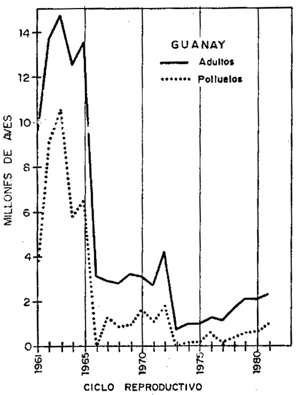
La evaluación de poblaciones de aves guaneras desde hace veinte años, mediante el método del censo gráfico, demuestra que el incremento de la población se halla en relación directa al éxito en cada ciclo reproductivo y la posterior supervivencia de polluelos; por esta razón se considera que el incremento de aves adultas se realiza a base de los polluelos del ciclo reproductivo anterior que sobrevivieron un año. Anteriormente ya se dijo que el éxito reproductivo, y en este caso, la supervivencia de polluelos se halla íntimamente ligado a la disponibilidad de las fuentes de alimentación; cuando estas fuentes de alimentación escasean, ocurren mortandades de adultos y juveniles. A base de estas consideraciones se elaboró la Tabla 6; en ella se puede apreciar que de los 20 años analizados en doce de ellos hubo incremento. Los incrementos mayores, con 4.45, 1.79 y 1.95 millones de aves fueron en los años 1961/62, 1964/65 y 1971/72, respectivamente. En los años restantes, los incrementos fueron de menor consideración. En cambio, durante los otros ocho años no consecutivos hubo mortalidades de adultos y polluelos, siendo los más graves los ocurridos en 1963/64, 1965/66 y 1972/73 con 3.35, 12.13 y 4.66 millones, respectivamente. Estas mortalidades concuerdan con los años en que ocurrieron anomalías oceanográficas en el mar peruano a causa del Fenómeno “El Niño”. Con respecto a los polluelos se notó las más altas mortalidades durante los años 1962/63, 1963/64, 1964/65 y 1965/66 con 10.70, 12.84, 4.22 y 8.10 millones respectivamente.
En 1979/80 hubo una mortalidad de 0.65 millones de adultos y 1.31 millones de polluelos.
Incremento y mortalidad de guanay (Tabla 7, Fig. 8):
Los estimados de la población de guanay, evaluada de 1960–1981, permitió conocer mejor que el guanay estuvo sujeto a fluctuaciones de consideración a causa de incremento en unos años y mortalidad en otros.
Los mayores incrementos en la población de guanay se produjeron durante los ciclos reproductivos de 1961/62, 1971/72 y 1977/78 con 45, 58 y 47%, respctivamente, incrementos menores ocurrieron durante los ciclos reproductivos de 1968/69, 1973/74, 1975/76 y 1978/79 con 12, 21, 25 y 26%, respectivamente. Estos incrementos estarian indicandor que existe un mecanismo de compensación en la población de guanay, porque estos incrementos se produjeron antes y después de períodos con mortalidades altas.
Estos descensos en los niveles poblacionales debidos a mortalidad ocurreron principalmente a causas de alteraciones del medio ambiente marino, principalmente; 1972/73 con mortalidades del 77 y 80% de la población, respectivamente; los períodos dode los porcentajes de mortalidad no fueron tan altos, estuvieron asociados a los altos volúmenes de captura de anchoveta para la industria, que disminuyó considerablemente y en forma gradual la disponibilidad de anchovetas para alimento de guanay, lo cual inclusive no permitió la recuperación del nivel poblacional después de cada mortalidad.
La población de guanay en 1980/81 representó sólo el 16% de la que existió en 1962/63. La reproducción en cada ciclo reproductivo aparentemente fue exitosa, a excepción de los años con perturbaciones ambientales en la que no hubo reproducción, pero después de concluída la reproducción los polluelos no llegan a sobrevivir al año de edad, produciéndose altos porcentajes de mortalidad por la escasez de alimento (principalmente anchoveta). Estas mortalildades ocurrieron en 13 años no consecutivos, con porcentajes de 70 a 100% de mortalidad de polluelos; razón por la que el nivel poblacional de guanay se mantiene bajo.
Incremento y mortalidad de piquero (Tabla 8, Fig. 8):
En la década del 60, los mayores incrementos de la población de piquero se produjeron en 1964/65, 1966/67 y 1968/69 con 32, 30 y 48%, respectivamente; pero también se produjeron mortalidades, notandose las más altas mortalidades de adultos en 1962/63, 1963/64, 1965/66 y 1967/68 con 8, 23, 64 y 10%, respectivamente; y la mortalidad de polluelos fueron muy altas llegando al 100% a excepción de los años en que se produjeron incrementos.
Durante la década del 70 se produjo incrementos superiores al 35% en los ciclos reproductivos 1973/74, 1975/76, 1977/78 y 1978/79, además hubo incrementos de 8 y 15% en 1970/71 y 1971/72, respectivamente. La mortalidad más alta ocurrió en 1972/73 con 55% de la población total y con 7, 9, 19 y 4% para los años 1974/75, 1976/77, 1979/80 y 1980/81, respectivamente.
En la década del 70 las mortalidades de los polluelos también fueron muy altas, a excepción de los años en que se produjeron incrementos, durante los cuales se observa cero de mortalidad.
Incremento y mortalidad de alcatraz o pelícano (Tabla 9, Fig. 8):
De las tres especies principales de aves guaneras, el alcatraz o pelícano fue la única especie que no fue afectada en forma duradera por los fenómenos ambientales y los altos volúmenes de captura de anchoveta para la industria. Después de cada descenso poblacional causado por los cambios ambientales, ésta se recuperó rápidamente, como lo demuestran los altos porcentajes de incrementos que inclusive en algunos casos como en 1973/74 y 1978/79 llegaran a 105 y 107%, respectivamente.
La mortalidad de adultos fue alta en los ciclos reproductivos de 1963/64 y 1972/73 con 71 y 63%, respectivamente. En cambio, la mortalidad de polluelos fue alta en la mayoría de los años, lo que demostraría que la población adulta se mantuvo en fluctuación pero siempre con un ritmo ascendente, superando en forma amplia los niveles poblacionales de la década del 60.
 |
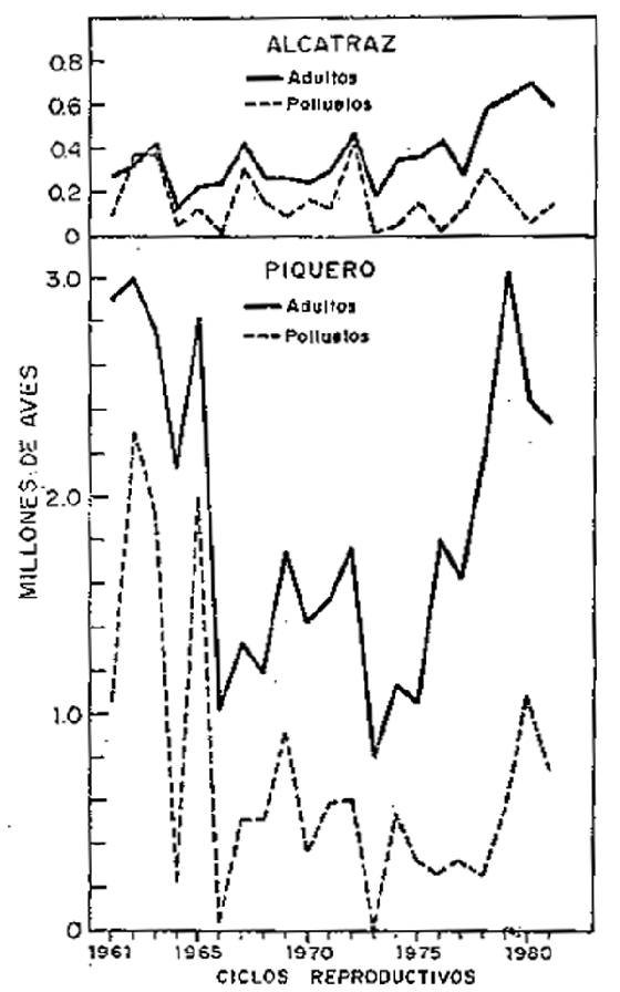 |
| Fig. 5.- Guanayes adultos y polluelos en cada ciclo reproductivo. | Fig. 6.- Población de Alcatraz y Piquero adulto y polluelos en cada ciclo reproductivw. |
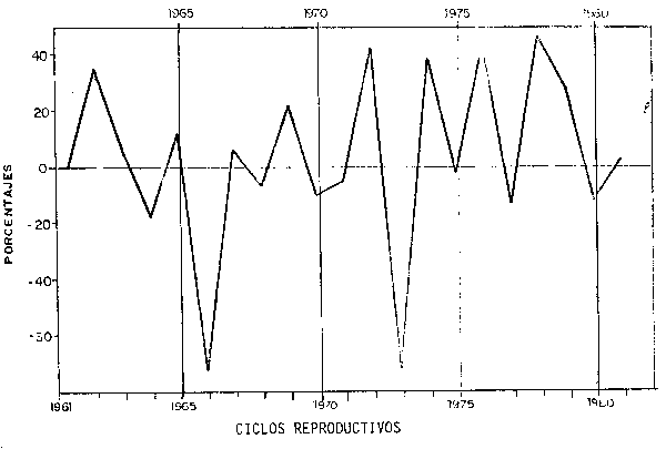
Fig. 7.- Incremento y Mortalidad de la población de aves graneras.
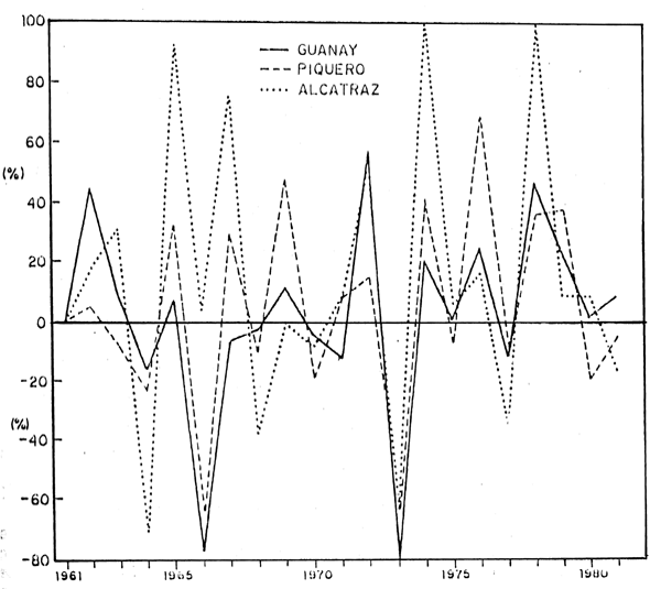
Fig. 8.- Incremento y mortalidad por especies en (%)
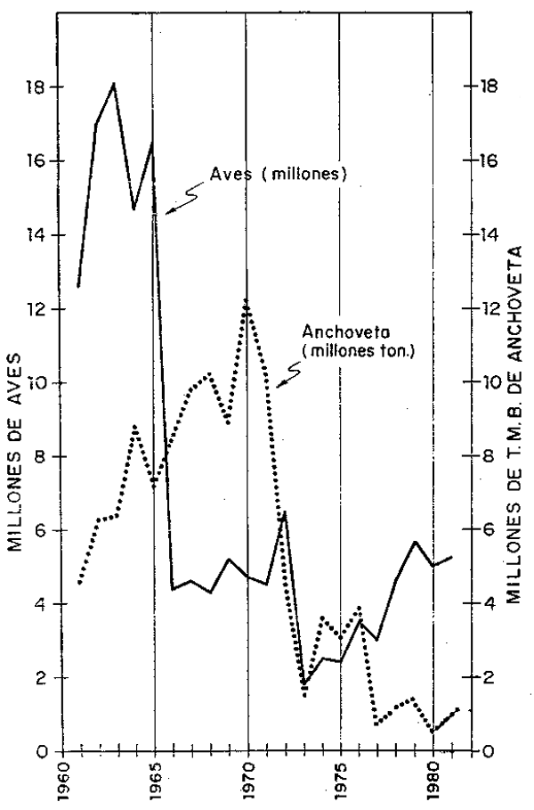
Fig. 9.- Población de aves guaneras (millones de individuos) y monto total de captura de anchoveta (en millones de ton.)
LAS AVES Y LA DISPONIBILIDAD DE ANCHOVETA
El recurso anchoveta desempeñó un papel muy importante en el desarrollo de poblaciones de aves por constituir la anchoveta el principal elimento de estas aves. Por esta razón, la mayor o menor disponibilidad del recurso anchoveta influyó directamente en las fluctuaciones de los niveles poblacionales de las aves.
De las estadísticas de captura anual de anchoveta se puede deducir que en la década del 60 aumentó la proción de este recursor tomada por la pesquería, no así la tomada por las aves que comenzaron a descender de 18 millones en 1963 hasta 4.31 millones de aves en 1968; por el contrario, la captura anual de anchoveta llegó a su máximo en 1970 con más de 12 millones de TMB.
En la década del 70, a consecuencia de las anomalías del medio ambiente marino ocurrido en 1972/73 y la sobrepesca de anchoveta en la década del 60 y comienzos del 70, la disponibilidad de anchoveta para alimento de las aves e inclusive para la pesquería, fue escasa. Al respecto Tsukayama (en prensa) hace una descripción secuencial de la pesquería de la anchoveta en el Perú. Aduciendo que en los últimos años el recurso anchoveta ha sido reemplazado por otros recursos íctocos. Jordón, Csirke y Tsukayama (1978) opinan que frente a la escasez de anchoveta se produjeron fenómenos de compensación, o sea, incremento de otros recursos.
CONCLUSIONES
Se han analizado datos de censos gráficos de las poblaciones de aves guaneras, con particular énfasis en los ciclos reproductivos 1974/75 – 1980/81.
En este período de la población de aves varión de 2.46 a 5.21 millones de aves notándose una lenta recuperación del nivel poblacional; sin embargo, la pesquería y los trastornos ambientales marinos siguen siendo factores limitantes en el desarrollo de poblaciones de aves guaneras.
En cuanto a la composición por especies, el piquero (Sula variegata) sigue predominando sobre el guanay (Phalacrocoraz bougainvillii) y pelícano o alcatraz (Pelecanus thagus).
El recurso anchoveta sigue siendo escaso para alimento de las aves e inclusive para la pesquería industrial.
En la década del 70, la población más alta fue 6.47 millones en 1971/72 contituido por 66, 27 y 7% de guanay, piquero y alcatraz o pelícano, respectivamente. El nivel más bajo de 1.81 millones se observó durante el Fenómeno “El Niño” de 1972, donde se observaron procentajes de 46, 44 y 9% de guanay, piquero y alcatraz, respectivamente. En los siguientes años se nota una lenta recuperación, llegando a 1980/81 con 5.21 millones de aves, compuesta por 45, 44 y 11% de piquero, guanay y alcatraz o pelícano, respectivamente.
Estos dos principales factores arriba citados, además de causar descensos en el nivel poblacional, han ocasionado considerables cambios en la composición por especies.
En el descenso poblacional, la especie guanay fue la más afectada; en cambio, el piquero y alcatraz han recuperado prácticamente su nivel poblacional, porque el problema de la escasez o poca disponibilidad de anchoveta para estas dos últimas especies fue solucionado cambiando la alimentación hacia otras especies ícticas.
AGRADECIMIENTOS
Expreso mi más sincero agradecimiento a la Biólogo Isabel Tsukayama por el interés demostrado en la elaboración del presente trabajo y las acertadas sugerencias; de la misma forma agradezo a Pesca Perú Fertilizantes (antes Servicio Nacional de Fertilizantes), especialmente al Dr. Demóstenes Cabrera por las facilidades brindadas en la obtención de información de los censos gráficos de aves guaneras y al personal de la Unidad de Dibujo por la preparación de las figuras. Finalmente, agradezo a la Sra. Isabel Delgado de Risso por el mecanografiado del manuscrito original de este trabajo.
REFERENCIAS
Avila, E. 1954. Potencial deyectiva del guanay (Ph. bougainvillii). Bol.Cient.Cia.Admora.Guano. 1(2):22–49.
Compañla administradora del Guano. 1946. 37a Memoria del directorio de la Compaña Administradora del Guano, correspondiente al año económico de 1945.
Compañla. 1954. El guano. Cia.Admora.Guano. 1–30.
Compañla. 1955. 47a Memoria del directorio correspondiente al ejercicio 1955.
Corporación Nacional de Fertilizantes. 1964. Memoria de la Corporación Nacional de Fertilizantes correspondiente al año 1964.
Fuentes, H. 1969. Las poblaciones de las aves guaneras después Especiales Inst.Mar. Perú-Callao. IM-54:1–18.
Gamarra, D.L. 1955. Ensayo sobre la zoonomía de la aves guaneras del Perú. Bol.Cia.Admora.Guano II:73–121.
Gamarra, D.L. 1964a. Las fluctuaciones en la población de las aves guaneras en la costa peruana. Bol.Cia.Admora.Guano. 2(12) 2 Epoca:3–12.
Gamarra, D.L. 1964b. Las fluctuaciones de la población de palmipedas marinas productoras del guano del Perú. Memoria de Fertilizantes correspondiente al año 1964.
Jordán, 1963. Resultados de los censos gráficos de las aves guaneras efectuados en noviembre de 1960 y enero de 1962. Callao, Inf.Inst.Recurs.Mar. 12:1–21.
Jordán. 1964. Las emigraciones y mortalidad de las aves en invierno y otoño de 1963. Callao, Inf.Inst.Invest.Recurs.Mar. 27:1–31.
Jordán, R. y H. Fuentes. 1964. Resultados de los censos gráficos de las aves guaneras efectuados durante el ciclo reproductivo 1962/63. Callao, Inf.Inst.Invest.Recurs.Mar. 22:1–15.
Jordán. 1966. Las poblaciones de aves guaneras y su situación actual. Informe Inst.Mar PerúCallao. 10:1–44.
Jordán, R., J. Csirke y I. Tsukayama. 1978. Situación de los recursos anchoveta, sardina, jurel y caballa a junio de 1978. Informe Inst.Mar Perú-Callao. 56:1–32.
Murphy, R.C. 1954. El guano y la pesca de anchoveta. Cia.Admora.Guano. Informe Oficial al Supremo Gobierno. 1–39.
Tovar, H. 1978. Las poblaciones de aves guaneras en los ciclos reproductivos de 1969/70 a 1973/74. Informe Inst.Mar Perú-Callao. 45:1–13.
Tovar, H. y L. García. 1982. Las poblaciones de aves guaneras durante “El Niño” de 1957. Boletin de Lima. 22:34–46, año 4de julio de 1982.
Tovar, H. y L. Galarza. (En prensa). Cambios en el régimen alimentario de guanay (Phalacrocorax bougainvillii lesson).
Tovar, H. (En prensa). Fluctuaciones mensuales de las poblaciones de aves guaneras durante “El Niño” de 1972.
Tsukayama, I. (En prensa). Recursos pelágicos y sus pesquerias en el Perú.
Vogt, W. 1942. Informe sobre las aves guaneras. Bol.Cia.Admora.Guano. II(8):9–28.
Vogt, W. 1942. Informe sobre las aves guaneras. Bol.Cia.Admora.Guano. II(9):6–48.
Vogt, W. 1942. Informe sobre las aves guaneras. Bol.Cia.Admora.Guano. II(10):5–40.
by
J. Alheit,1 B. Alegre,2 V.H. Alarcón,2 and B. Macewicz3
1 Programa Cooperativo Peruano-Alemán de Investigación Pesquera (PROCOPA), IMARPE, Apartado 22, Callao, Perú
2 Instituto del Mar del Perú, Apartado 22, Callao, Perú
3 Southwest Fisheries Center, P.O. Box 271, La Jolla, CA 92038, U.S.A.
* Publication No. 7 of PROCOPA
Resumen
Recientemente se han revelado yarias características esenciales de la biología reproductiva de la anchoveta peruana (Engraulis ringens) y ahora pueden ser comparadas con aquellas de la anchoveta del norte (E. mordax). Así como la anchoveta del norte, la anchoveta de sistema de afloramientos de Perú desova en forma parcial, depositando varias series de huevos a lo largo del año. Ahora se dispone de datos de series de tiempo sobre la fecundidad parcial de varias sub-poblaciones de ambas especies. La variabilidad de la fecundidad parcial es alta dentro de cada año y de un año a otro. En ambas especies, la fecundidad parcial aumenta a medida que aumenta la latitud. Fuera de las épocas principales de desove (Agosto-Septiembre y Enero) la fecundidad parcial de la anchoveta peruana disminuye. Durante El Niño de 1976, la fecundidad parcial de E. ringes disminuyó considerablemente. Esto se atribuye a las condiciones desfavorables de alimentación. La fecundidad parcial de E. capensis frente al sudoeste de Africa se encuentra dentro del rango de los valores de las otras dos especies. La frecuencia del desove fue determinada por exámenes histólogicos de los ovarios para observar la incidencia de folículos post-ovulatorios. La fracción de hembras maduras que desovan por día fue de 16% en 1961 frente a Perú y 14.5% en 1980 frente a California. Todos los parámetros reproductivos investigados son muy similares en ambas especies, indicando una relación filogénetica estrecha. La importancia de determinar la fecundidad parcial y la frecuencia del desove se basa en su uso para “el método de la producción de huevos” que fue desarrollado recientemente para estimar la biomasa desovante de anchoveta. Este método ha sido aplicado con suceso en los stocks de anchovetas frente a California y Perú. Se discuten los resultados, ventajas y futuras aplicaciones de este método para otras especies de peces pelágicos que forman cardúmenes tales como sardinas.
INTRODUCTION
Recently, a new method, the ‘Egg Production Method’, was developed by the Southwest Fisheries Center, California, to estimate the spawning biomass of anchovies (Parker, 1980; Stauffer and Picquelle, 1980). This method requires the determination of reproductive parameters like batch fecundity and spawning frequency, i. e. the fraction of mature females spawning per day.
The determination of batch fecundity and spawning frequency for multiple spawning pelagic fish, like the anchovy, posed several problems which were solved by Hunter and Goldberg (1980). In traditional methods, size — frequency diagrams of oocytes were established and it was assumed that fecundity could be determined by counting the number of all oocytes contained in the most advanced mode. Hunter and Goldberg (1980) discussed the problems involved in this method. Instead, they determined the batch fecundity by counting the number of hydrated oocytes in the ovaries. This method takes much less time and yields a higher precision than traditional methods. For the determination of the spawning frequency, Hunter and Goldberg (1980) used the incidence of postovulatory follicles in anchovies. They were able to age postovulatory follicles and to determine the day when a particular female had spawned. All these studies were carried out on the northern anchovy (Engraulis mordax). Recently, the same methods were applied successfully, to the Peruvian anchovy (E. ringens) (Alheit et al., in prep.; Santander et al., in prep.).
Time series are available now on the batch fecundity of the Peruvian and the northern anchovy. The data were partly gained from previous studies using traditional methods (MacGregor, 1968; Laroche and Richardson, 1980) and from samples collected in Peru during the seventies which were processed recently.
The objectives of this study are (1) to compare the time series on batch fecundity of the two anchovy species, (2) to compare for both species the data on batch fecundity and spawning frequency gained by the new methods, and (3) to discuss their use for estimates of spawning biomass of multiple spawning pelagic fish.
This study was a cooperative effort of the Southwest Fisheries Center, California, the Instituto del Mar del Peru and the Peruvian-German Fisheries Research Project (PROCOPA) which is financed by the German Agency of Technical Cooperation (GTZ).
METHODS
The batch fecundity of the Peruvian anchovy samples collected in the seventies was determined by macerating the connective tissue of the ovaries in Gilson's fluid (Simpson, 1951), a process which releases the oocytes. The size of the oocytes was measured and the number of oocytes in the most advanced mode was determined by means of probability paper (Cassie, 1954). The recent batch fecundity data for the Peruvian and northern anchovy were gained by using hydrated oocytes (Hunter and Goldberg, 1980). The methods used for determining the batch fecundity of other anchovy populations presented here are described n MacGregor (1968) for the northern anchovy in 1951-60, in Laroche and Richardson (1980) for the northern population of the northern anchovy and in LeClus (1979) for the anchovy off South West Africa (E. capensis ). The spawning frequency was determined according to the methods described by Hunter and Goldberg (1980), Stauffer and Picquelle (1980) and Alheit et al. (in prep.).
| Lot | Species | Sub-population | Year | Month | Sample Size | Size Range of fish (gonad-free weight in g) | Mean Nr Oocytes per g female | S.D. | Mean Nr. Oocytes per g Ovary | S.D. | r | Slope | Y-intercept |
|---|---|---|---|---|---|---|---|---|---|---|---|---|---|
| 1 | E. ringens | central | 1970 | Jan | 19 | 15.2–40. | 7 123 | + 2719 | 375 | + 147 | .685 | 1 048 | -16 627 |
| 2 | " " | central | 1973 | Sep | 26 | 15.1–38.7 | 5 998 | + 2728 | 410 | + 172 | .564 | 746 | -8 527 |
| 3 | " " | " " | 1974 | Jan | 8 | 22.8–43.2 | 9 231 | + 1938 | 489 | + 133 | .554 | 847 | -13 125 |
| 4 | " " | " " | " | Feb | 8 | 32.2–44.2 | 6 011 | + 999 | 326 | + 91 | .126 | 667 | -13 506 |
| 5 | " " | " " | " | Aug | 12 | 17.7–41.3 | 7 067 | + 2049 | 484 | + 157 | .717 | 1 517 | -31 194 |
| 6 | " " | " " | " | Sep | 9 | 21.0–48.4 | 8 233 | + 1577 | 410 | + 142 | .692 | 705 | -8 814 |
| 7 | " " | " " | " | Oct | 18 | 16.3–54.5 | 6 607 | + 2295 | 268 | + 110 | .799 | 558 | -8 804 |
| 8 | " " | " " | 1976 | Aug | 32 | 6.8–34.5 | 11 606 | + 5447 | 415 | + 143 | .813 | 424 | -227 |
| 9 | " " | " " | " | Aug | 11 | 15.0–34.5 | 7 686 | + 1800 | 414 | + 149 | .509 | 360 | 1257 |
| 10 | " " | southern | 1973 | Sep | 19 | 14.1–21.7 | 7 205 | + 3125 | 395 | + 122 | .614 | 1 352 | -17 490 |
| 11 | " " | " " | 1974 | Aug | 23 | 9.0–41.3 | 6 432 | + 2351 | 446 | + 175 | .831 | 1 087 | -13 545 |
| 12 | " " | northern +) central | 1981 | Aug/Sep | 437 | 15.0–38.0 | *) | 580 | .+ 139 | 806 | 981 | -10 279 | |
| 13 | E. ringens | central | 1981 | Aug/Sep | 254 | 15.0–38.0 | *) | 637 | + 134 | .769 | 1 213 | -14 745 | |
| 14 | " " | northern | " | Aug/Sep | 183 | 15.0–38.0 | *) | 502 | + 103 | .883 | 824 | -7 655 | |
| 15 | E. mordax1) | central | 1951-1960 | 19 | 9.3–32.1 | 12 253 | + 2737 | 606 | + 151 | .795 | 670 | -1 247 | |
| 16 | " " | " " | 1978 | 23 | 9.3–31.9 | *) | 389 | + 141 | .511 | 528 | -2 790 | ||
| 17 | " " | " " | 1979 | 44 | 9.3–28.1 | *) | 438 | + 150 | .784 | 881 | -7 917 | ||
| 18 | " " | " " | 1980 | 33 | 17.11+) | *) | 444 | + 80 | .903 | 624 | -2 933 | ||
| 19 | " " | " " | 1981 | 127 | 14.75+) | *) | 601 | + 180 | .873 | 872 | -3 711 | ||
| 20 | " " | " " | 1982 | 109 | 16.54+) | *) | 606 | + 151 | .724 | 852 | -4 061 | ||
| 21 | " " | northern2) | 1977 | 17 | 14.4–31.3 | 7 137 | + 3997 | 869 | + 213 | .860 | 1 494 | -12 015 | |
| 22 | E. capensis3) | 1977 | 14 | 17.5–24.3 | 4 491 | + 851 | 644 | + 153 | .451 | 1 542 | -18 657 |
| 1) From MacGregor (1968) 2) From LaRoche and Richardson (1980) | 3) From LeClus (1979) |
| *) Parameter not calculated as hydrated oocytes were used | +) Average weight |
RESULTS
Time series on fecundity of Peruvian anchovy. 14 different data sets on fecundity of the Peruvian anchovy are available (Table 1). They originate from different years, months and areas. There are no trends recognizable for the mean number of oocytes per gram female, however, some interesting features can be pointed out. Only one data set, January 1970, was collected before the crash of the Peruvian anchovy in 1972. This value is relatively, but not particularly low. The data set from August 1976 was collected during an ‘El Niño’ year. The collection includes many very small mature females between 7 and 15 g. To make this data more comparable, another data set comprising only the larger specimens (11 fish) is presented separately. The values from August 1976 lie just within the range of the other data sets. There are two data sets from the south, but they are not outliers. The only remarkable feature is the difference between the relatively low values from the seventies and the high values from 1981. This difference is probably not caused by the use of different methods. In 1981, two data sets were taken, one from the central region and one from the northern region. The one from the central region is with 637 eggs per gram female; much higher than the 499 eggs per gram female from the northern region. This might not necessarily be a regional difference, as the northern samples were, on average, collected two weeks later than the central samples. It could be that the value for the number of eggs per gram female is very flexible and can change very fast towards the end of the spawning season. In general, one can observe a decrease of the mean number of eggs per gram female after the main spawning periods in August/September and January, e. g. in 1974 and 1981. The number of oocytes per gram ovary, does not show any trend. Only the value for the large data set from August 1976 lies outside of the range of the other values. However, this high value is caused, solely, by the high number of very small mature females. The mean number of oocytes per gram ovary is not given for 1981, as this value changes during the process of hydration.
| The relationship between batch fecundity and female weight (ovary-free) was investigated further by using the geometric mean regression (Ricker, 1973) Whereas all other data from the Peruvian anchovy have a relatively high Y — intercept, only the data from August 1976 have a positive and a relatively low negative value (Table 1). Differences between the 14 data sets become more obvious from the regression lines in Figures 1–3. They are presented in three different groups whereby the whole data set from August 1981 serves as a reference line. Group 1 includes all the data collected during the yearly peak spawning periods in August/September and January (Figure 1). These regression lines are not too different from each other. The second group comprises the ‘El Niño’ data from August 1976 and data sets collected at February 1974 and October 1974, outside of the yearly main spawning periods ( Figure 2). These data sets have in common a relatively low batch fecundity for females larger than 30 g. The third group demonstrates regional differences. Obviously the fecundity values from the southern Peruvian anchovy stock are higher than in the central and northern stock. Although the data sets were taken in different years, they indicate, that the batch fecundity increases with increasing latitude (Figure 3). | 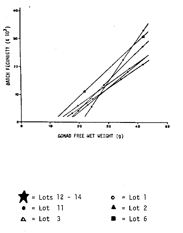 Fig. 1. Batch fecundity of E. ringens populations. Geometric mean regression of number of eggs per spawn on gonad-free female wet weight. |
| Comparison of fecundity of different
anchovy species. Batch fecundity data
are available for the Peruvian anchovy,
the northern anchovy and the anchovy from
South West Africa. The values for the
mean number of oocytes per gram female
from the northern anchovy and the anchovy
off South West Africa lie within the
range of the Peruvian data (Table 1).
The only exception is the high value for
the northern population of the northern
anchovy. From 1978 to 1982 the values
of the central population of the
northern anchovy increased steadily from
389 to 606 eggs per gram female weight.
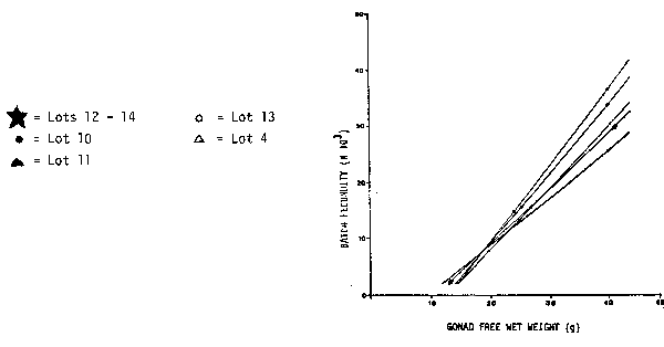
The regression lines of the central population of the northern anchovy are relatively uniform (Figure 4). However, the regression line of the northern population is very distinct and demonstrates that females with more than 15 g weight have a much higher batch fecundity than in the central population. Again, as in Peru, the batch fecundity of anchovy populations increases with increasing latitude. |
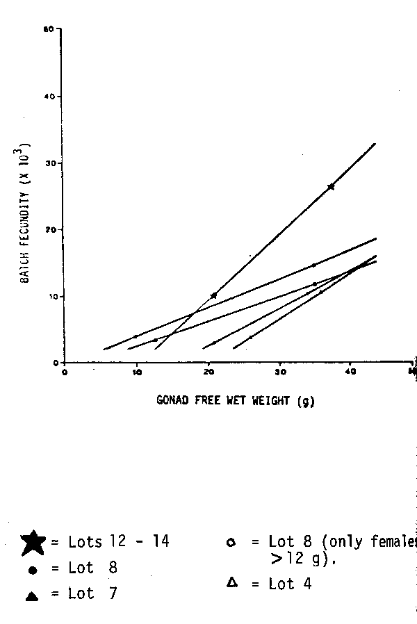
Fig. 2. Batch fecundity of E. ringens populations. Geometric mean regression of number of eggs per spawn on gonad-free female wet weight. |
| Fig. 3. Batch fecundity of E. ringens populations. Geometric mean regression of number of eggs per spawn on gonad-free female wet weight. | |
|
|
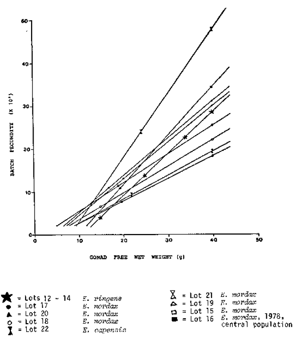
Fig. 4. Comparison of Different Species. Batch fecundity of anchovy populations. Geometric mean regression of number of eggs per spawn on gonad-free female wet weight.
Spawning frequency. The fraction of mature females spawning per day was determined for the Peruvian anchovy in August/September 1981. As a purse seiner was used to collect the adult anchovies, fish samples could be obtained at any time of the day and two data sets were established, one giving the fraction of females which spawned one day before being collected and the other one giving the fraction of females which had spawned two days before being sampled. These two spawning fractions were 17.26% and 14.81%, respectively (Alheit et al., in prep.).
The agreement of these two data sets demonstrates the validity of the method introduced by Hunter and Goldberg (1980). The spawning frequency determined for the Peruvian anchovy by combining these two data sets was 16.04%. That means every day during August/September 1981, on average, 16.04% of the mature females were spawning, or in other words, a female of the central and northern Peruvian stock spawned, on average, every 6.2 days a new batch of eggs. The spawning frequency recorded for the northern anchovy in 1981 was 14.5% (Stauffer and Picquelle, 1980) a value very similar to that one of the Peruvian anchovy.
Use of data on reproductive biology for estimates of spawning biomass. Batch fecundity and spawning frequency are two of the five parameters used for determining the spawning biomass of anchovies by means of the ‘Egg Production Method’ (Parker, 1980; Stauffer and Picquelle, 1980). So far, this method has been applied in California and Peru. The results of the Californian survey from 1980 (Stauffer and Picquelle, 1980) and from the Peruvian survey from 1981 (Santander et al., in prep.) are listed in Table 2.
| Peru 1981 | California 1980 | |||
|---|---|---|---|---|
| &xcirc | CV&xcirc | &xcirc | CV&xcirc | |
| Daily egg production in survey area | 6.985.103 | 0.2586 | (10.50)* | 0.103 |
| Average female weight (g) | 25.84 | 0.0259 | 17.50 | 0.0547 |
| Fraction of females | 0.564 | 0.0459 | 0.476 | 0.120 |
| Batch fecundity (eggs/female) | 15 401 | 0.0427 | 7 788 | 0.0749 |
| Spawning frequency | 0.160 | 0.0588 | 0.145 | 0.125 |
| Spawning biomass (million tons) | 1.295 | 0.2739 | 0.859 | 0.225 |
* This value is the number of eggs per ton.
DISCUSSION
The comparison of the batch fecundity data of different anchovy populations demonstrates clearly the high plasticity in batch fecundity of anchovies. There is a high variability in batch fecundity within years and between years as the Peruvian and Californian data show. One can only speculate about what causes this variability. Sufficient quantities of the right food are probably a very important condition for a fish to build up a high batch fecundity as argued by Bagenal (1978) and Wootton (1979). This might be indicated by the low fecundity values during the ‘El Niño’ year 1976 when feeding conditions were unfavourable for the Peruvian anchovy.
Tsukayama and Alvarez (1980) reported that during the “El Niño” 1976 growth of the Peruvian anchovy was retarded and that the mean size of mature females was considerably less than in normal years. They suggested that the high proportion of small females would reduce the fecundity of the whole population. This hypothesis is confirmed by the data presented here. Population fecundity in 1976 was further reduced by the much lowered fecundity values of the larger females in comparison to other years (Figure 2). This lowered population fecundity is caused by the combined effect of a high proportion of small females and of large females having a lower batch fecundity than in normal years and certainly exerted a negative influence on subsequent recruitment.
The importance of the determination of batch fecundity and spawning frequency is based on their applications in the ‘Egg Production Method’ to estimate the spawning biomass of anchovies. The main advantages of the ‘Egg Production Method’ are its high precision and that it needs relatively little ship time. It consists of 5 biological parameters and error estimates can be determined for each of them (Table 2). To date, it has been applied four times in the Californian upwelling system (1980–1983) and once in Peru (1981).
Up to now, it was applied only to anchovies. However, it is suitable for other multiple spawning pelagic fish species, too. Recently, postovulatory follicles have been identified and aged for the Peruvian sardine (Sardinops sagax sagax) (Alarcon et al., in prep.), a vital step towards the application of the ‘Egg Production Method’ for sardines.
REFERENCES
Alarcón, V.H., S.R. Goldberg and J. Alheit. (In preparation). Histología de folículos post-ovulatorios de la sardina, Sardinops sagax sagax, del Perú. Bol.Inst.Mar Perú, Callao.
Alheit, J., V.H. Alarcón and B.J. Macewicz. (In preparation). Spawning frequency and sex ratio in the Peruvian anchovy, Engraulis ringens.
Bagenal, T.B. 1978. Aspects of fish fecundity. In Ecology of Freshwater Fish Production (S.D. Gerking, ed.). Blackwell Scientific Publications, Oxford. 520 p.
Cassie, R.M. 1954. Some uses of probability paper in the analysis of size frequency distributions. Aust.J.Mar.Freshwater Res. 5:513–522.
Hunter, J.R. and S.R. Goldberg. 1980. Spawning incidence and batch fecundity in northern anchovy, Engraulis mordax. Fish.Bull.U.S. 77:641–652.
Laroche, J.L. and S.L. Richardson. 1980. Reproduction of northern anchovy, Engraulis mordax, off Oregon and Washington. Fish.Bull.U.S. 78:603–618.
Le Clus, F. 1979. Fecundity and maturity of anchovy Engraulis capensis off South West Africa. Fish.Bull.S.Afr. 11:26–38.
MacGregor, J.S. 1968. Fecundity of the northern anchovy, Engraulis mordax Girard. Calif.Fish Game. 54:281–288.
Parker, K. 1980. A direct method for estimating northern anchovy, Engraulis mordax, spawning biomass. Fish.Bull.U.S. 78:541–544.
Ricker, W.E. 1973. Linear regression in fishery research. J.Fish.Res.Board Can. 30:409–434.
Santander, H., J. Alheit and P.E. Smith. (In preparation). Estimación de la biomass desovante de la anchoveta Peruana, Engraulis ringens, del stock central y norte en 1981 usando el “Método de Producción de Huevos”. Bol.Inst.Mar Perú, Callao.
Simpson, A.C. 1951. The fecundity of the plaice. Fishery Invest., Lond., Ser. 2. 17:27 p.
Stauffer, G.D. and S.J. Picquelle. 1980. Estimates of the 1980 spawning biomass of the central subpopulation of northern anchovy. Southwest Fisheries Center Administrative Rep. No. LJ80–90.
Tsukayama, I. and M.A. Alvarez. 1981. Fluctaciones en el stock de anchovetas desovantes durante las temporadas reproductivas de primavera 1964–1978. Bol.Inst.Mar Perú, Callao. Volumen extraordinario:50–54.
Wootton, R.J. 1979. Energy costs of egg production and environmental determinants of fecundity in teleost fishes. pp. 133–159. In Fish Phenology: anabolic adaptiveness in teleosts (P.J. Miller, ed.). Academic Press, London. 443 p.
by
1 International Center for Living Aquatic Resources Management (ICLARM), MCC P.O. Box 1501, Makate, Metro Manila, Philippines
2 Instituto del Mar del Perú, Apartado Postal 22, Callao, Perú
* ICLARM Contribution No. 145, PROCOPA Contribution No. 14.
Resumen
Se han examinado en detalle datos de longitud-captura mensual de anchoveta peruana (Engraulis ringens) correspondientes a la region Norte, usando los programas de computadora ELEFAN I y III (Electronic LEngth Frequency ANalysis). ELEFAN I proporcionó para cada uno de los años, desde 1961 a 1979, valores similares de L∞y K de la ecuación de crecimiento de Von Bertalanffy. Se muestra que ocurren oscilaciones estacionales en el crecimiento, los cuales son cuantificados.
El programa ELEFAN III, que permite la aplicación de diferentes formas del análisis de población virtual en base a datos de longitud-captura, fue empleado para obtener series de tiempo, sobre una base mensual, de los siguientes parámetros: reclutamiento (R), stock desovante (S) y biomasa total (B). También se presentan y discuten series de tiempo de capturas mensuales (C) y de valores derivados (loge (R/S) y F = C/B).
INTRODUCTION
For about 10 years (1962–1971), the Peruvian anchoveta (Engraulis ringens, Jenyns [Fam: Engraulidae]) supported the largest single-species fishery in the world, with annual catches in excess of 12 million tonnes. Present catches are lower, but still make this species a very important aquatic resource (see contributions in Glantz and Thompson, 1981). The anchoveta has been much studied, and indeed, most methods available for assessing exploited fish stocks have been applied to the anchoveta, often by the very scientists who developed these methods (Boerema et al., 1967; Schaefer, 1967; Gulland, 1968; IMARPE, 1970, 1972, 1973, 1974, 1977a).
The present paper continues this tradition in that it reports on the application to the anchoveta of a newly developed set of methods for the investigation of exploited fish stocks. The set of methods are incorporated in the ELEFAN (Electronic LEngth Frequency ANalysis) programs developed at ICLARM* which are applied to catch-at-length data from the Northern Region of Peru and covering the years 1961 to 1979.
Of the three available, the two ELEFAN programs used were:
- ELEFAN I (Pauly and David, 1981; Pauly et al., 1980); this program is used for the extraction of growth parameters from length-frequency (L/F) or catch-at-length (C/L) data, using an algorithm which allows for seasonal growth oscillations to be considered and which provides results that are fully reproducible.
- ELEFAN III (Pope et al., MS, cited in Pauly, 1982); this program was used to run two types of length-structured virtual population analysis (VPA) on catch-at- length data, and to obtain estimates of recruitment, standing stock and fishing mortality on a monthly basis.
The analyses performed and the conclusion reached here are, for reasons to be discussed further below, quite preliminary. This paper should be read with emphasis on the methodology used, rather than on the numerical values of the results obtained.
MATERIAL AND METHODS
Raw data
The data used for all analyses presented here originally consisted of monthly length- frequency data collected from March 1961 to December 1979 by staff of the Instituto del Mar del Perú (IMARPE) in the ports of Chicama, Chimbote, Samanco and Casma (of these Chimbote accounts for more than 80% of anchoveta landings in the Northern Region). The data analyzed here thus pertain to the northern stock of anchoveta (see IMARPE, 1970 for comments on the status of anchoveta stocks off the Peruvian-Chilean coast).
The sampling procedures for length-frequency samples generally followed those given in Saetersdal and Valdivia (1964), who presented data suggesting that for the stretch of coastline ranging from the Northern to the Central Regions, within port variability of the length-frequency samples was less than variability due to different sampling periods. Monthly samples representative of the northern stock as a whole were obtained by pooling daily samples representing more than 30% of the landings, and most of the fishing areas covered by the fleet. Generally, one single sample was taken from each vessel sampled; the sample consisted of the contents of a two-liter container, of which all anchoveta were measured and weighed. The monthly samples representative of the monthly catches were then raised to the catch.
* The first version of ELEFAN III was written by J.G. Pope at Lowestoft, England.
During periods when the commercial fishery was closed, length-frequency data were obtained from 1972 on by sampling during “EUREKA Surveys”, and other scientific surveys and cruises. Here, the samples (taken after each haul) were raised to the total catch made during the survey or cruise (see IMARPE, 1972, 1974 for brief accounts of the EUREKA and other surveys and cruises).
The data used all refer to total length, and are grouped in 0.5 cm classes. For the analysis of growth, the data were regrouped into 1 cm classes to obtain a number of length classes of about 20 or less, which is optimum for analysis with ELEFAN I (Pauly et al., 1980).
The full data set used here extended to the period before 1961 and beyond 1979 will be published later, along with an analysis more detailed than that presented here.
Growth
The analysis of length-frequency and catch-at-length data using ELEFAN I is based on the following assumptions (adapted from Pauly and David, 1981):
- the samples used represent the population investigated,
- the seasonally oscillating version of the von Bertalanffy Growth Function (VBGF) describes the average growth of the fish,
- all fish in the samples have the same length at the same age and therefore differences in length can be attributed to differences in age.
Another assumption in Pauly and David (1981), namely “that the growth patterns are the same from year to year” need not apply here as the estimation of growth parameters was performed separately for each year. The last of the three assumptions above certainly does not apply as anchoveta of different sizes can very well be expected to have the same age. The anchoveta, however, is not a long-lived fish, and, as will be shown below, the bulk of a cohort goes through the exploited phase within less than two years, with the result that fish hatched during say, a given month remain identifiable as a group through- out most of their exploited life span (see Saetersdal and Valdivia, 1964 and Fig. 1).
Put briefly, the ELEFAN I program does the following (adapted from Pauly and Ingles, 1981):
- restructures the length-frequency samples that have been entered such that “peaks” are attributed “positive points”, and the “troughs” separating peaks “negative points”,
- calculates from the positive points of the peaks of all samples entered a sum named “available sum of peaks” (ASP, analogous to the total variance of parametric methods),
- traces a series of growth curves starting from the bases of the peaks, and projects these curves backward and forward in time such as to hit the other samples in the data set and recording all “points” (positive and negative) “hit” by a curve,
- identifies the curve and hence, the growth parameters - which, by passing through most peaks and avoiding most troughs, best “explains” the peaks in the sample set. This curve will have scored the highest number of points, whose sum is called on the “explained sum of peaks” (ESP, analogous to the explained variance of parametric methods).
Given the validity of the assumptions presented above, ELEFAN I can be used to obtain growth parameters that are completely objective, i.e., in which no assumptions as to the age composition of the catch have been incorporated prior to analysis (Pauly and David, 1981).
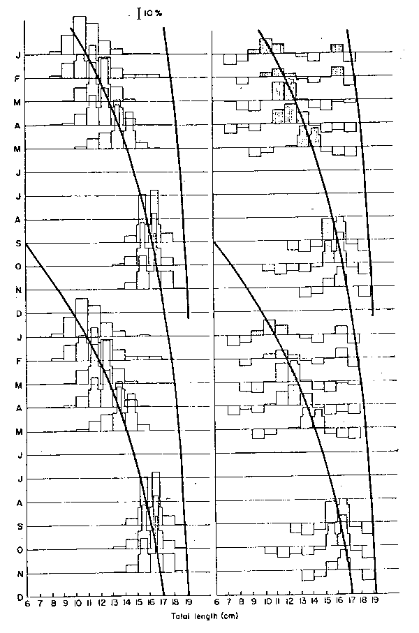
Fig. 1. (Left) Catch-at-lenth data for anchoveta, fitted with a growth curve using ELEFAN I; note “doubling up” of 1970 data to allow for a longer growth curve to be drawn.
(Right) Restructured length-frequency data as used internally by ELEFAN I; note that, through the restructuring process, peaks have become positive “points” (shaded bars) while the troughs separating peaks have become negative “points” (open bars).
The seasonally oscillating version of the VBGF used here has the form

where:
Lt is the length at age t,
L∞ the asymptotic length,
K a growth constant,
to the “age” at which length is zero if the fish always grew according to the equation,
C is a dimensionless constant expressing the intensity of the growth oscillations,
and ts is the time (with respect to t=0) at the beginning of a sinusoidal growth oscillation of period one year (Pauly and Gaschütz, 1979; Gasch tz et al., 1980).
In ELEFAN I, the estimation of ts is replaced by the estimation of a Winter Point (WP), defined as
| ts + 0.5 = WP | …2 |
which expresses (as a fraction of the year) the time during which growth is slowest. It should be mentioned here that ELEFAN I, being based on length-frequency data (rather than length-at-age data) does not allow for the estimation of to, hence of absolute ages; all “ages” used internally by the program are relative ages, expressed in relation to an arbitrary birthdate (the 1st of January).
ELEFAN I was applied to the available data for the years 1969 to 1979, yielding 19 independent estimates of growth parameters.
Virtual Population Analysis
The ELEFAN III program, in its latest version (Pope, et al., MS) consists of 4 main routines:
- a routine to convert length-frequency data into catch-at-length data (not used here, as IMARPE data had already been converted),
- a routine to run a conventional age-structured VPA (here termed VPA I), as discussed, e.g., in Pope (1972),
- a routine to run a VPA-version of Jones' (1979, 1981) length-cohort analysis (here termed VPA II, see below), and
- a routine to run an age-structured VPA on catch-at-length data arranged such that they produce the functional equivalents of cohorts (here termed VPA III, see below).
VPA I is based on the equation

where Ni is the population (in number) at the beginning of time period i, while Ci and Fi are the catch and the fishing mortality during that same time period i. Usually equation (3) is solved (iteratively) backwards, starting from a “terminal population” (Nt) estimated from

where Ft is the (assumed) terminal fishing mortality and Ct the terminal catch, while M is the natural mortality which is generally assumed constant throughout (Pope, 1972).
Generalizing equation (3) to any time interval (°) gives

This equation is a functional equivalent of Jones (1979, 1981) equation for length cohort analysis and can be used to run a VPA on catch-at-length data starting from
| Nt = Ct · Zt/Ft | …6 |
and estimating ° from

i.e., by calculating using the VBGF, the time needed to grow from the lower (L1) to the upper (L2) limit of a length class (see Jones, 1981). Equation (5) is used here, instead of the original length-cohort analysis proposed by Jones (1979, 1981) because as shown by Pauly (in press) the VPA version of Jones' method produces results which are insensitive to the width of the length classes into which the catch data are grouped; Pope et al. (MS) and Pauly (in press) give more details on this method.
It must be mentioned, however, that the method does not provide estimates of standing stock and fishing mortality pertaining to a given cohort (as does VPA I); rather the method provides estimates of the population of fish and the fishing mortalities that must have existed for the recorded catches to have been generated (Jones 1981). The method is therefore at its best when catch data from longer time periods are grouped such as to simulate equilibrium conditions.
For this paper, we have grouped the available monthly catch data into years, and thus report estimates of annual recruitment, standing stock and fishing mortality.
VPA III is a version of VPA I performed on “cohorts” obtained by superimposing growth curves, drawn at monthly intervals, onto a set of catch-at-length data, the catch pertaining to each “cohort” and month being simply that part (obtained by addition and interpolation) of a monthly catch contained between two growth curves (see Fig. 2).
For such cohorts to consist of fish recruited at the same time, the growth curves used for “slicing up” a cohort must be obviously as close to the true growth curve of that cohort as possible, which among other things makes it imperative that a seasonally oscillating curve be used since, as shown in Pauly and Ingles (1981) and Pauly (1982), virtually all fish species display seasonally oscillating growth.
In reality, not all fish of a given cohort have the same growth parameters, and it can be expected that some fish will “leave their cohort” because they grow either faster or slower than predicted by the mean growth curve of their cohort. Such differences in growth rate should here have the effect of somewhat smoothing month to month variations in the estimates of fishing mortality and derived parameters.
The VPA III routines of ELEFAN III were applied to the available catch-at-length data using the growth parameters given in Table 1. The small year-to-year differences in the values of the growth parameters caused a slight overlap of some “cohorts” (i.e., some of the catch data were used twice), and small gaps (i.e., some of the catch data were not included in any cohort.) This source of error could have been avoided by using the same growth parameters throughout. This, however, would have caused misidentification of some cohorts.
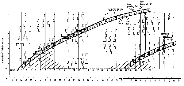
Fig. 2. Schematic representation (not to scale) of VPA III as implemented in ELEFAN III. Two “cohorts” (#1 and 23) are shown; they are defined by the growth parameters of the growth curves on their upper and lower boundaries, and by that part of the catch (black histograms) comprised between these boundaries. The terminal catches are shown. Note (partial) compensation of fish leaving a “cohort” (due to slower or faster growth) by fish from neighboring cohorts. Length at recruitment (Lr) is defined by smallest fish in catch.
Table 1: Growth parameters of Peruvian anchoveta (Engraulis ringens, northern stock) as estimated by means of the ELEFAN I computer program.
| Year | L∞ (cm) | K (per year) | WPa | Ca | ESP/ASP |
|---|---|---|---|---|---|
| 1961 | 19.65 | 1.26 | (0.6) | (0.2) | 0.572 |
| 1962 | 20.75 | 1.16 | 0.8 | 0.35 | 0.513 |
| 1963 | 18.95 | 1.39 | 0.8 | 0.3 | 0.439 |
| 1964 | 20.70 | 1.22 | 0.6 | 0.23 | 0.588 |
| 1965 | 20.75 | 1.21 | 0.6 | 0.4 | 0.503 |
| 1966 | 20.75 | 1.30 | 0.65 | (0.3) | 0.475 |
| 1967 | 20.05 | 1.36 | 0.9 | 0.3 | 0.655 |
| 1968 | 20.95 | 1.205 | 0.96 | 0.32 | 0.655 |
| 1969 | 20.95 | 1.19 | 0.6 | 0.23 | 0.570 |
| 1970 | 19.55 | 1.39 | 0.8 | 0.3 | 0.832 |
| 1971 | 20.75 | 1.30 | (0.75) | (0.3) | 0.532 |
| 1972 | 20.70 | 1.27 | 0.7 | 0.3 | 0.421 |
| 1973 | 20.95 | 1.20 | 0.5 | 0.3 | 0.598 |
| 1974 | 21.85 | 1.20 | 0.5 | 0.2 | 0.504 |
| 1975 | 21.25 | 1.16 | 0.5 | 0.2 | 0.581 |
| 1976 | 21.25 | 1.31 | 0.85 | 0.3 | 0.420 |
| 1977 | 21.05 | 1.31 | 0.8 | 0.3 | 0.519 |
| 1978 | 20.75 | 1.2 | 0.6 | 0.4 | 0.787 |
| 1979 | 20.75 | 1.215 | 0.82 | (0.3) | 0.458 |
 | 20.65 | 1.26 | 0.70 | 0.30 | - |
| s.d. | 0.681 | 0.073 | 0.147 | 0.061 | - |
| C.V. (in %) | 3 | 6 | 21 | 20 | - |
| 95% confidence interval | ±0.31 | ±0.033 | ±0.070 | ±0.031 | - |
a values in brackets are set values; they were not used for the computation ofmeans or confidence intervals.
Preliminary computations suggest that the errors in the recruitment and standing stock estimates are of about ±15%, which is quite acceptable given the uncertainties involved in such important parameters as natural mortality and terminal fishing mortality (see below).
A value of M=1.2 (annual basis) was used throughout, for both VPA II and VPA III. This value has been used previously by several authors (e.g. Ricker, 1975, p. 197), and was obtained as the intercept of a plot of Z (obtained from catch curves) on effort (T. Burd, pers. comm. in Schaefer, 1967).
A terminal fishing mortality Ft=1.2, corresponding with M=1.2 to an exploitation rate (E=F/(F+M) of 0.5 was used to estimate terminal populations for both VPA II (using Equation 6) and VPA III (using Equation 4). Since E=0.5, as will be shown below, was reached in the mid-60's, the terminal populations have been underestimated in the earlier years, and overestimated in the later years.
Size at recruitment was defined as 4 cm, i.e., slightly less than the 5 cm value used by other authors. It must be considered that, in any case, true catches of “peladilla” (small anchoveta) are underestimated because the fish often disintegrate before processing.
The mean size at first maturity (i.e., the size distinguishing adults from juveniles) used here was a constant set at 11 cm. This is slightly lower than the 12 cm figure suggested by other authors (Saetersdal and Valdivia, 1964; Murphy, 1972). This size was chosen to account for cases (during El Niño events) where fish reach maturity at much reduced sizes (Tsukayama and Alvarez, 1981).
Biomasses were estimated by multiplication of computed population size (by length) with fish weights, the fish weights being estimated from
| W=a . Lb … | 8 |
Values of a=0.0065 and b=3 were used throughout, with length expressed in centimeters and W in grams. At this stage of our analysis, we made no efforts to account for within and between years variations of the length/weight relationships, although we are aware that such variations occur (IMARPE, 1976, 1977a, 1977b, 1980, 1981, 1982), and may cause under- or over-estimates of standing stock.
All computer-based analyses were performed on a Radio Shack TRS 80 Model III micro- computer.
RESULTS
Growth
Table 1 gives 19 estimates of the values of the growth parameters L, k, C and WP for the period 1961 to 1979. As might be seen, there was no trend over time in any of the parameters and it can therefore be stated that the parameters describing the growth in length of the northern stock of the Peruvian anchoveta have been more or less constant from the period 1961 to 1979, despite large changes in biomass (this does not preclude changes in the growth in weight, see above).
The mean value of C=0.30 suggests that the growth of anchoveta oscillates seasonally in sinusoidal fashion, and that it is, during the warmest summer month, 30% higher than it would be if no oscillations occurred. Conversely, the growth of anchoveta is reduced in winter, down to a 30% reduction during the coldest month; “winter” as perceived by the anchoveta occurs at WP=0.70 ± 0.07, corresponding to the 12th of September (± 26 days). The temperature data in Zuta and Urquizo (1972) show that sea surface temperatures off Peru oscillate in sinusoidal fashion, with most common values for minima and maxima occurring in September and March, respectively.
The range of the oscillation of mean monthly temperature, moreover, is 3 to 6°C; these values correspond well to the mean value of C (which expresses the intensity of the growth oscillations) reported here (Fig. 3).
Two important points must be borne in mind when considering these results:
- the values of C and WP were extracted from length-frequency data, yet match very well the values that would have been predicted on the basis of the temperature regime off Peru alone and
- the oscillations reported here are generally too faint to be perceived, let alone quantified using standard methods (i.e., eye-fitting) for the analysis of length-frequency data.
VPA II
Table 2 summarizes the results obtained using VPA II (Table 3 gives an example, pertaining to 1968, of the output obtained from ELEFAN III).
VPA III
The estimates of recruitment (R), adult stock (S), values of loge (R/S), the catches, total biomass and estimates of fishing mortality are presented as monthly values for the period 1961 to 1979 in Figs. 4 to 9.
The values of loge (R/S) in Fig. 6 are in fact values of loge (Ri/Si-1), i.e., the recruitment of a given month was plotted against the adult biomass of the preceding month. Fig. 14 in Saetersdal and Valdivia (1964) suggests that 4 cm fishes are generally between 1 and 2 months old.
| Fig. 3.Values of C (expressing the intensity ofseasonal growth oscillations) plotted against ° T (expressing the difference between warmest and coldest mean monthly water temperature) in a number of tropical and temperate fishes. The shaded area, referring to the anchoveta, is based on the C values in Table 1 and range of ° T values in Zuta and Urquizo (1972). Note that the seasonal oscillations in the growth of anchoveta conform to the general pattern established for other fishes by Pauly and Ingles (1981). | 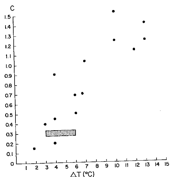 |
| Year | Recruitmentb | Catchc | ēd |  e e |  c, f c, f |
|---|---|---|---|---|---|
| 1960 | 212 | - | - | - | - |
| 1961 | 317 | 1314 | 0.39 | 0.77 | 1713 |
| 1962 | 295 | 2194 | 0.39 | 0.75 | 2908 |
| 1963 | 509 | 1908 | 0.40 | 0.81 | 2365 |
| 1964 | 353 | 3429 | 0.47 | 1.07 | 3197 |
| 1965 | 434 | 2290 | 0.46 | 1.01 | 2258 |
| 1966 | 479 | 2903 | 0.52 | 1.33 | 2177 |
| 1967 | 579 | 3837 | 0.33 | 0.58 | 6581 |
| 1968 | 547 | 4351 | 0.36 | 0.68 | 6418 |
| 1969 | 626 | 3293 | 0.51 | 1.26 | 2616 |
| 1970 | 483 | 4028 | 0.46 | 1.03 | 3909 |
| 1971 | 127 | 3289 | 0.49 | 1.14 | 2887 |
| 1972 | 359 | 910 | 0.38 | 0.72 | 1264 |
| 1973 | 159 | 321 | 0.48 | 1.11 | 289 |
| 1974 | 114 | 744 | 0.35 | 0.64 | 1157 |
| 1975 | 132 | 852 | 0.34 | 0.61 | 1391 |
| 1976 | 22.5 | 566 | 0.61 | 1.88 | 302 |
| 1977 | 8.72 | 135 | 0.51 | 1.24 | 109 |
| 1978 | 61.6 | 425 | 0.51 | 1.26 | 336 |
| 1979 | - | 321 | 0.46 | 1.00 | 320 |
a The January 1962 and February 1962 catches were added to the 1961 catch (March toDecember) to obtain 1961 figures comparable to those of the other years.
b The catch of a given year was used to infer recruitment the preceding year; this is anapproximation (see text); recruitment refers to number of 4 cm fish (x 109).
c In tonnes (x103)
d Obtained from E=number of fish caught/number of fish dying of all causes; latternumber is approximated by the recruitment itself, since all fish recruited finally die.
e Obtained as F=(M/(1-E))-M.
f Obtained from  =catch in weight/mean fishing mortality.
| <<<<< VPA 2 RESULTS FOR ENGRAULIS RINGENS 1968 >>>>> | |||
|---|---|---|---|
| LENGTH | CATCHES | POPULATION | FISH. MORTALITY |
| 19–19.5 | 3 | 6 | 1.2 |
| 18.5–19 | 17 | 25.768 | 7.37504 |
| 18–18.5 | 106 | 143.361 | 10.9724 |
| 17.5–18 | 1056 | 1274.2 | 16.9331 |
| 17–17.5 | 4349 | 8008.53 | 13.5436 |
| 16.5–17 | 11183 | 18433 | 10.8091 |
| 16–16.5 | 19061 | 40308.8 | 8.12607 |
| 15.5–16 | 36190 | 81861.2 | 8.09872 |
| 15–15.5 | 36383 | 126845 | 5.07618 |
| 14.5–15 | 34147 | 172461 | 3.57291 |
| 14–14.5 | 12637 | 198366 | 1.14295 |
| 13.5–14 | 5840 | 218118 | .503711 |
| 13–13.5 | 2809 | 235119 | .237521 |
| 12.5–13 | 4008 | 253521 | .334135 |
| 12–12.5 | 3614 | 271744 | .29685 |
| 11.5–12 | 4647 | 291220 | .376049 |
| 11–11.5 | 4272 | 310547 | .340511 |
| 10.5–11 | 3933 | 329733 | .309429 |
| 10–10.5 | 2788 | 347927 | .217158 |
| 9.5–10 | 3135 | 366598 | .24216 |
| 9–9.5 | 2372 | 384620 | .18188 |
| 8.5–9 | 2204 | 402564 | .168023 |
| 8–8.5 | 1381 | 419754 | .104829 |
| 7.5–8 | 1007 | 436612 | .0762341 |
| 7–7.5 | 492 | 452980 | .0371878 |
| 6.5–7 | 186 | 469052 | .0140503 |
| 6–6.5 | 47 | 484987 | 3.54992E–03 |
| 5.5–6 | 5 | 500878 | 3.77701E–04 |
| 5–5.5 | 17 | 516780 | 1.28429E–03 |
| 4.5–5 | 8 | 532671 | 6.04442E–04 |
| 4–4.5 | 4 | 548556 | 3.02256E–04 |
| TOTAL | CATCH = 197901 | MEAN E = .360767 | MEAN F = .677251 |