![]()
![]()
![]()
FIGURE 4.1
Schematic presentation of the soil erosion and productivity model
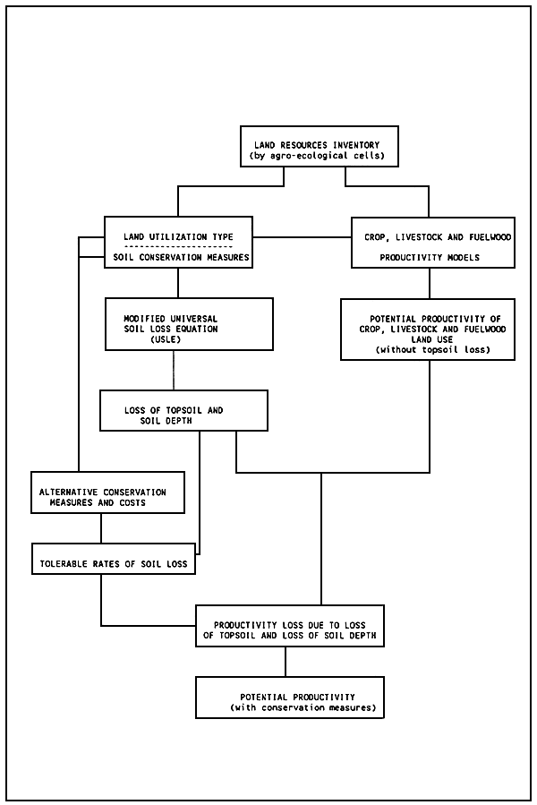
This chapter describes the soil erosion and productivity model, which quantifies implications of alternative land uses in terms of topsoil loss due to erosion and its impact on the productivity of land under different assumed soil conservation measures. The model operates on the climatic and soil resources inventories described in Technical Annex 1. and in Chapter 3. Details of the model are described in Technical Annex 2.
The methodology for the estimation of topsoil loss is essentially based on a modified Universal Soil Loss Equation (USLE): Wischmeier and Smith (1978). The topsoil loss is subsequently converted into productivity loss with or without specific soil conservation measures. The methodology is schematically shown in Figure 4.1. and comprises the following steps:
Identification of land utilization types (LUTs), as defined for crop, livestock and fuelwood productivity models.
Determination of (USLE) factors for soil erosion: i.e. rainfall erosivity factor, soil erodibility factor, vegetation/crop cover factor, management factor and physical protection factor.
Application of USLE to quantify (LUT-specific) topsoil loss.
Establishing the relationships (equations) between loss of yield and loss of topsoil, and classifing soil units according to their susceptibility of yield loss due to loss of topsoil.
Application of equations from (iv) to estimate productivity loss in relation to productivity potentials as quantified by the land use (crop, livestock, fuelwood) productivity models.
Derivation of productivity estimates, tolerable soil loss and costs for alternative conservation measures.
The Universal Soil Loss Equation (USLE) equates soil loss per unit area with the erosive power of rain, the amount and velocity of runoff water, the erodibility of the soil, and mitigating factors due to vegetation cover, cultivation methods and soil conservation. It takes the form of an equation where all of these factors are multiplied together:
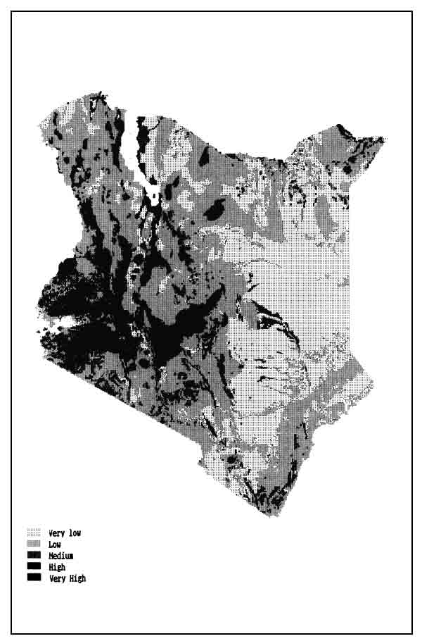
FIGURE 4.2
Generalized map of potential erosion hazard
| A = R × K × LS × C × P | (4.1) |
where:
| A: | Annual soil loss in t/ha |
| R: | The rainfall erosion factor to account for the erosive power of rain, related to the amount and intensity of rainfall over the year. It is expressed in units described as erosion index units. |
| K: | The soil erodibility factor to account for the soil loss rate in t/ha per erosion index unit for a given soil as measured on a unit plot which is defined as a plot 22.1 m long on a 9% slope under a continuous bare cultivated fallow. It ranges from less than 0.1 for the least erodible soils to approaching 1.0 in the worst possible case. |
| LS: | A combined factor to account for the length and steepness of the slope. The longer the slope the greater the volume of runoff, the steeper the slope the greater its velocity. LS = 1.0 on a 9% slope, 22.1 m long. |
| C: | A combined factor to account for the effects of vegetation cover and management techniques. These reduce the rate of soil loss, so in the worst case when none are applied, C = 1.0 while in the ideal case when there is no loss, C would be zero. |
| P: | The physical protection factor to account for the effects of soil conservation measures. In this report conservation measures are defined as structures or vegetation barriers spaced at intervals on a slope, as distinct from continuous mulches or improved cultural techniques which come under the management techniques. |
The USLE equation has been modified by separating the two elements of the cover and management factor, C as follows:
| C*: | The vegetation cover factor. This accounts only for the effects of the natural vegetation or crop canopy (including leaf litter and residues accumulating during the life of the crop). |
| M: | The management factor. This accounts for tillage methods, the effects of previous crop residues, previous grass or bush fallows, and applied mulches. |
The soil loss equation therefore becomes:
| A = R × K × LS × (C* × M) × P. | (4.2) |
Equation 4.2 is used in the model to estimate topsoil loss under specified vegetation/crop cover and management conditions for each land utilization type (LUT) as defined in the crop, livestock and fuelwood productivity models (Technical Annexes 4, 5 and 6). These estimates in turn are related to productivity losses and conservation needs (Figure 4.1).
Each of the factors making up the soil loss equation 4.2 is quantified in turn, for a specified land use (LUT) or alternative land uses. Attributes of land utilization types for crops, pasture (livestock) and fuelwood are given in Tables S.2, 6.2 and 7.2 respectively. The soil loss quantification procedure is presented in Technical Annex 2. Figure 4.2 presents a generalized map of potential erosion hazard. This map combines of the erosivity factor (R), the erodibility factor (K) and the slope factor (LS).
TABLE 4.1
Slope-cultivation association screen
| Land utilization type | Low | Level of inputs Intermediate | High |
| Dryland crops without soil conservation measures | <30% | <30% | <16% |
| Dryland crops with soil conservation measures | <30% | <30% | <30% |
| Wetland crops without soil conservation measures | <5% | <5% | <2% |
| Wetland crops with soil conservation measures1 | <30% | <30% | <30% |
| Coffee, tea, fuelwood and pasture with and without soil conservation measures | <45% | <30% | <45% |
1 For wetland crops, terracing is required.
The effect of soil erosion can be measured in different ways according to the kind of damage suffered. In the model (Figure 4.1), the estimate is based on short-term losses in crop production due to erosion of fertile topsoil, and long-term losses in land productivity due to truncation of the soil profile and consequent reduction of available water. No account is taken at this stage in the model development of possible damage to lowlands by flooding and silt deposition, or of the possible benefit from the deposition of fertile silt on alluvial plains, or increase in workability constraints due to changes in terrain characteristics.
In the model, permissible slopes for various land uses under different levels of inputs circumstances have been defined as model variables, and these are given in Table 4.1. The critical slope values in the slope-land use association screen define the upper slope limits to cultivation, and they may be modified as appropriate.
Further, the model takes into account the loss in crop production by soil erosion through:
the removal of topsoil which, in many soils, is the source of most or all the nutrient fertility; and
reducing the overall depth of the soil profile so that eventually the soil water holding capacity and foothold capacity are reduced to a point where it limits yields.
An acceptable rate of soil erosion is considered to be one that over a specified number of years (e.g. 25, 50 or 100):
does not result in a crop yield reduction of more than a specified amount due to loss of topsoil; and
does not result in more than a specified proportion of land being downgraded to a lower class of agricultural suitability due to soil depth reduction.
These two criteria are not interdependent, so that acceptable rate of soil loss is taken as the lower of the two alternatives. The model therefore provides a framework for assessing tolerable soil loss, based on its likely impact on crop yields and the future availability of cultivable land.
The soil erosion and productivity model (Figure 4.1) is linked to crop, livestock and fuelwood productivity models which provide the assessments of land suitabilities and the associated yield potentials for the estimation of tolerable soil loss.
Soils differ in their susceptibility to loss of productivity as the topsoil is eroded. The differences are related to the depth of the topsoil and the amount of nutrient fertility or presence of unfavourable conditions in the subsoil.
Loss of productivity due to topsoil loss can be largely compensated by the use of manure and fertilizer, and low rates of soil erosion are compensated to some extent by the formation of new topsoil. The rate of topsoil formation can vary from < 0.25 mm/year in dry and cold environments to > 1.5 mm/year in humid and warm environments (Hammer 1981; Hudson 1981). Topsoil formation at the rate of 1 mm/year is equivalent to an annual addition of 12 t/ha. Therefore, the rate of topsoil formation has been considered as a factor in the model in assessing loss of productivity and tolerable soil losses. Regeneration capacities of soils used in the model in calculating net loss of topsoil are given in Table 4.2 by moisture and thermal regimes.
Based on experimental evidence (Stallings 1957; Barr 1957; Lal 1976a, 1976b, 1976c; Higgins and Kassam 1981) and analytical data from Kenya Soil Survey (KSS 1975, 1976, 1982b), soil units of the Exploratory Soil Map of Kenya have been classified according to their susceptibility to productivity loss with loss of topsoil, and on the presence of other unfavourable subsoil conditions (Table 4.3). These rankings of susceptibility of the soils are related to actual yield losses, by inputs level, through a set of linear equations given in Table 4.4. The reduced impact of topsoil loss under intermediate and high levels of inputs is due to the compensating effect of fertilizers at their normal rates of use. It is assumed that the benefit of fertilizers is less on the more susceptible soils because of their more unfavourable subsoil conditions.
The tolerable loss rate, for a given soil unit and specified amount and time scale of yield reduction, is calculated in the model as follows:
| TL = {(Ra/Rm × 100 × B × Dt) + 3T} / T | (4.3) |
| where: | TL = | tolerable loss rate (t ha-1 year-1) |
| Ra = | acceptable yield reduction (%) | |
| Rm = | yield reduction (%) at the given inputs level when the effective topsoil is all lost | |
| B = | bulk density of the soil (g/cm3) | |
| Dt = | depth of effective topsoil (cm) | |
| T = | time (years) over which yield reduction is acceptable. |
| LGP | Thermal zone | ||||||||
| (days) | T1 | T2 | T3 | T4 | T5 | T6 | T7 | T8 | T9 |
| < 75 | 0.5 | 0.5 | 0.5 | 0.5 | 0.5 | 0.25 | 0.25 | 0.25 | 0.25 |
| 75 – 119 | 1.0 | 1.0 | 1.0 | 0.5 | 0.5 | 0.25 | 0.25 | 0.25 | 0.25 |
| 180 – 269 | 1.5 | 1.5 | 1.5 | 0.75 | 0.75 | 0.5 | 0.6 | 0.5 | 0.5 |
| > 270 | 2.0 | 2.0 | 2.0 | 1.0 | 1.0 | 0.5 | 0.5 | 0.5 | 0.5 |
Derived from Hammer (1981).
| Most susceptible | Intermediate susceptible | Least susceptible |
| Acrisols, except Humic Arenosol | Arenosols | Chernozems |
| Ferralic Cambisols | Cambisols, except Ferralic Cambisols | Fluvisols |
| Ferralsols, except humic Ferralsols | Gleysols | Histosols |
| Ironstone soils | Greyzems | Humic |
| Lithosols | Humic Acrisols | Andosols |
| Planosols | Humic Ferralsols | Mollic |
| Rendzinas | Kastanozems | Andosols |
| Solonchaks | Luvisols | Vertisols |
| Solonetz | Nitisols | |
| Phaeozems | ||
| Regosols | ||
| Vitric Andosols | ||
| Xerosols | ||
| Yermosols |
TABLE 4.4
Relationships between topsoil loss and yield loss
| Soil susceptibility ranking | Levels of inputs | Equation |
| Least susceptible | Low | Y = 1.0 X |
| Intermediate | Y = 0.6 X | |
| High | Y = 0.2 X | |
| Intermediate susceptible | Low | Y = 2.0 X |
| Intermediate | Y = 1.2 X | |
| High | Y = 0.4 X | |
| Most susceptible | Low | Y = 7.0 X |
| Intermediate | Y = 5.0 X | |
| High | Y = 3.0 X |
Y = productivity loss in percent:
X = topsoil loss in cm.
The rate of soil formation by rock weathering is extremely slow, up to 0.025 mm/year on volcanic rocks in humid areas, and < 0.01 mm/year on basement complex rocks in semi-arid areas (Dunne, Dietrich and Brunego 1978). At the highest rate quoted by Dunne et oil.(1978), it would take 4,000 years to produce 10 cm of soil. Therefore, the rate at which the soil profile is deepened by rock weathering has not been considered as a factor in the model in assessing tolerable soil losses.
The estimation of the effect of soil depth reduction is based on the assumption that there is no significant loss of productivity until the soil becomes so shallow that shortage of moisture becomes a limiting factor. The critical depth varies according to crop and the climate. Once this critical depth is reached, productivity loss is linear until the soil becomes to shallow to produce any crop at all (Wiggins and Palma 1980). The critical points can be equated with land suitability class limits as follows (where depth is the limiting factor):
| VS/S: | Soil water becomes limiting and there is at least 20% decrease in yield potential |
| S/MS: | Soil water becomes limiting and there is at least 40% decrease in yield potential |
| MS/mS: | Soil water becomes limiting and there is at least 60% decrease in yield potential |
| mS/N: | Soil water becomes limiting and there is at least 80% decrease in yield potential. |
The suitability classes VS (very suitable), S (suitable), MS (moderately suitable), mS (marginally suitable) and N (not suitable) correspond to yield levels of > 80%, 60–80%, 4060%, 20–40% and < 20% of maximum attainable yield respectively.
If erosion takes place uniformly on soils of varying depth, the end result will be that some soils that had been marginally deep enough will become non-productive while others will become marginal. If the range of soil depths is known, the tolerable amount of soil loss can be gauged in terms of the amount of land that can be permitted to be lost to production.
In order to calculate tolerable soil losses, soil depth reduction is measured in terms of the proportion of the soils in a specified area that have become shallower than a given depth, as a result of erosion. The soils of the mapping units of the Exploratory Soil Map of Kenya (KSS 1982a) are assigned to 5 depth classes: shallow, < SO cm; moderately deep, 50–80 cm; deep, 80–120 cm; very deep, 120–180 cm; extremely deep, > 180 cm.
The rate of soil loss is related to the proportion of land whose soil has become shallower than a specified depth, by the following equations:
(a) Proportion (P, percent) of land downgraded to at least the next depth class:
| P = (SL × T)/(B × Dr) | (4.4) |
| where: | SL = | soil loss (t ha-1year-1) |
| T = | time (years) | |
| B = | bulk density of the soil (g/cm3) | |
| Dr = | depth range of the soil class (cm). |
(b) Proportion (P, percent) of land downgraded by more than one depth class:
| Soil depth class and change (cm) | Amount of land downgraded (% of class) at erosion rates (t/ha) of: | |||||||
| 5 | 10 | 25 | 50 | 75 | 100 | 200 | 400 | |
| From shallow (0–50) | ||||||||
| to bedrock (0) | 8 | 17 | 42 | 83 | 100 | |||
| From moderately deep (50–80) | ||||||||
| to shallow (0–50) | 14 | 28 | 70 | 100 | ||||
| to bedrock (0) | 0 | 0 | 0 | 0 | 42 | 100 | ||
| From deep (80–120) | ||||||||
| to moderately deep (50–80) | 10 | 21 | 52 | 100 | ||||
| to shallow (0–50) | 0 | 0 | 0 | 25 | 81 | |||
| to bedrock (0) | 0 | 0 | 100 | |||||
| From very deep (120–180) | ||||||||
| to deep (80–120) | 7 | 14 | 35 | 70 | 100 | |||
| to moderately deep (50–80) | 0 | 0 | 0 | 3 | 38 | 72 | 100 | |
| to shallow (0–50) | 0 | 0 | 22 | 100 | ||||
| to bedrock (0) | 0 | 78 | 100 | |||||
| From extremely deep (200–400) | ||||||||
| to very deep (120–180) | 2 | 4 | 9 | 19 | 28 | 38 | 76 | 100 |
| to deep (80–120) | 0 | 0 | 0 | 0 | 1 | 11 | 48 | 100 |
| to moderately deep (50–80) | 0 | 0 | 30 | 100 | ||||
| to shallow (0–50) | 0 | 17 | 92 | |||||
| to bedrock | 0 | 70 | ||||||
| Soil depth class | Susceptibility to yield loss of topsoil | ||
| Low | Intermediate | High | |
| Shallow1 | 3.0 | 3.0 | 3.0 |
| Moderately deep | 3.6 | 3.6 | 3.6 |
| Deep | 4.8 | 4.8 | 4.8 |
| Very deep | 7.2 | 7.2 | 7.2 |
| Extremely deep | 12.0 | 26.4 | 26.4 |
1 Assuming a minimum depth of 25 cm for crop production.
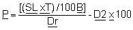 | (4.5) |
| where: | D2 = | difference (cm) between the lower limit of the depth class and the upper limit of the shallower class to which the land is downgraded |
| Dr = | depth range of the soil class (cm). |
Table 4.5 shows the proportions of land downgraded from given depth classes to shallower classes as a result of soil erosion at different rates over a 100 years period. The values in Table 4.5 are based on equations 4.4 and 4.5, and assume that soil depths are evenly distributed over the range in each depth class.
If a tolerable soil loss was set to allow 10% of each depth class to be downgraded by one class over 100 year period, this would give the following soil loss rates for each depth class (assuming 25 cm is the minimum soil depth that would allow crop production):
| Shallow (to 25 cm) | - 3 | t ha-1 year-1 |
| Moderately deep | - 3.6 | |
| Deep | - 4.8 | |
| Very deep | - 7.2 | |
| Extremely deep | - 26.8 |
Criteria for estimating soil loss tolerance are set according to the amount of yield loss that can be tolerated, or the proportion of the land that can be permitted to become shallower than a specified depth, over a specified time. The two basis for soil loss estimation do not interact, so when used in combination the tolerable soil loss would be the lower of the estimates.
An example of the soil losses that would give either a 50% yield reduction or soil depth reduction resulting in downgrading of 10% of each depth class, over a period of 100 years, is given in Table 4.6.
Three kinds of benifits can be obtained from soil conservation on cultivated land:
Long-term reduction or halting of decline in agricultural production or availability of good quality land.
Immediate or gradual increase in agricultural production.
Non-agricultural benefits such as improved dry season flow of rivers, reduced flooding and siltation of reservoirs, and reduced damage to infrastructure and farm land on lower slopes.
The soil erosion and productivity model essentially quantities the long-term benefits (i.e. reducing or preventing further losses of agricultural land and decline in crop yields) of seven soil conservation measures for alternative uses of land. It is envisaged that the model would be extended in the future to include an estimation of other agricultural and non-agricultural benefits implied in (b) and (c) above.
The seven types of conservation measures considered in the model are: cut-off drains, narrow-based terraces, bench terraces, converse terraces (“fanya juu” terraces), grass strips, trash-lines, and stone terraces. Of these, narrow-based terraces and grass strips are suitable for large farms, while all measures except narrow-based terraces are suitable for small farms. Bench terraces can be used on large farms, but the costs of making them wide enough for mechanical cultivation is high. Also, narrow-based terraces are applicable to slopes < 20%, whereas effectiveness of grass strips is reduced in low rainfall areas (LGP < 150 days) because of poor establishment. Also, trash-lines are subject to availability of crop residue whereas stone terraces are subject to availability of stones, and are feasible only on stony soils.
In the application of the soil erosion and productivity model (Figure 4.1), potential erosion losses for each desired land use (crop, livestock, fuelwood) is evaluated first on the assumption that no specific soil conservation measures are applied, i.e. protection factor P = 1. The results are compared with what is considered as acceptable rates of soil loss under the three levels of inputs circumstances, and then the required amount of conservation and associated costs are estimated.
The need for soil conservation is estimated from the protection factor (P) required to reduce soil erosion from its average rate on unprotected land to the tolerable rate estimated in Section 4.2.3. The average rate of erosion covers both the cultivated and the uncultivated parts of the crop and fallow period cycle, but the soil conservation measures described are only applied and maintained in the cultivated part of the cycle. If unacceptable rates of erosion are also occurring during the uncultivated part of the cycle, then additional protection will be needed.
The following example shows how conservation need is estimated in the model, for the cultivated part of the crop and fallow period cycle.
| Year | Annual soil loss (t/ha) | Total soil loss (t/ha) | |
| 1–4 | (Rest period) | 4 | 16 |
| 5 | (Crop 1st year) | 12 | 12 |
| 6 | (Crop 2nd year) | 18 | 18 |
| 7–10 | (Crop 3rd – 6th year) | 25 | 100 |
| Total soil loss over 10 years | 146 | ||
| Tolerable rate of soil loss over 10 years | 8 | 80 | |
Soil loss reduction needed is 66 t/ha (i.e. 146-80). The total soil loss over 6 years of the crop cycle is 130 t/ha, which has to be reduced by 66 t/ ha to 64 t/ha. The P factor needed to achieve this is 64/139 = 0.49.
The protective effect of conservation measures varies according to natural conditions soil, topography, climate - and the intensity of the measure, e.g. the interval between terraces.
The equations to calculate the required spacing for a given measure, when the relevant natural conditions and the required protection - P factor - are known, are given in Mitchell (1986). These equations form the basis of cost calculations in the model for the seven types of conservation measures listed above.
These conservation measures deal with cultivated land, and in the model their benefit is assumed to last only while the land is under cultivation. If excessive erosion is taking place during the uncultivated part of a crop-fallow period cycle, the most effective way to reduce it is by improving the grass cover. The first requirement for this is to reduce or eliminate the grazing pressure of livestock. Tables 4.7 and 4.8 (Technical Annex 2) show the percent grass cover at different times of the year, and assumed rates of regeneration of grass cover after cultivation, in relation to climate and grazing intensity. These can be used to estimate the effect on soil erosion of reducing the intensity of grazing.
Other possible causes of excessive erosion on uncultivated land are poor established grass due to low rainfall, and unfavourable soil conditions. These have not been explicitly incorporated in the model at this stage in its development, but possible measures to overcome them are: pasture improvement with fertilizers; planting of improved pasture species or broadcasting seed; use of lines of cut bushes to slow runoff to protect germinating grass seeds; use of small earth banks to trap water to encourage germination of broadcast seed (Critchly 1984).
The costs of conservation measures are given in terms of man-days of labour, and the proportion of land taken out of agricultural production by the measures. Where fertilizer is used, for example in establishing grass strips, the amount of fertilizer is specified. It is assumed that all materials used are locally available and therefore not explicitly costed.
Table 4.7 presents a generalized comparison of the characteristics, effectiveness and costs of the seven types of conservation measures considered in the model.
The appropriate conservation measure for a given set of circumstances is normally the cheapest that will achieve the required measure of protection. The costs presented in Table 4.7 are based on man-days of work for manual labour. These include initial costs and maintenance costs. Initial costs are mainly based on the horizontal interval between measures, whereas annual maintenance costs are derived as fixed percentage of the initial costs. In order to compare costs directly, the annual maintenance costs over the cultivated part of the 10-year crop and fallow cycle are converted to net present value using an interest rate of 10%.
Most conservation measures involve taking some land out of production. They vary according to the type of measure, and whether the plants used to protect the terrace banks and other structures have any production value.
TABLE 4.7
Economic aspects of soil conservation measures
| Type of measure and physical protection factor (P) | Slope (%) | Horizontal interval (m) | Height of risers (m) | Initial cost | Annual maintenance cost (mart-day/ha) | Proportion of land taken out of agriculture (%) | ||
| Construction (man-day/ha) | Grass planting (man-day/ha) | Fertilizer (kg/ha)1 | ||||||
| Cut-off drains P = 0.25–0.752 | >16 | - | - | 27 | - | - | 3 | - |
| <16 | - | - | 40 | - | - | 4 | - | |
| Narrow-based terraces P = 0.1–0.42 | 6 | 40 | 1.0 | 50 | 17 | 5 | 5 | 5 |
| 8 | 20 | 1.0 | 100 | 36 | 10 | 10 | 10 | |
| 16 | 10 | 1.6 | 200 | 51 | 15 | 20 | 15 | |
| 32 | 5 | 1.6 | 400 | 102 | 30 | 40 | 30 | |
| Bench terraces P = 0.05–0.152 | 12 | 8 | 1 | 1000 | 44 | 12 | 104 | 6 |
| 12 | 16 | 2 | 2000 | 44 | 12 | 204 | 6 | |
| 16 | 6 | 1 | 900 | 58 | 16 | 96 | 8 | |
| 16 | 12 | 2 | 1800 | 58 | 16 | 186 | 8 | |
| 24 | 4 | 1 | 750 | 88 | 24 | 84 | 10 | |
| 24 | 8 | 2 | 1500 | 88 | 24 | 159 | 10 | |
| 32 | 2.8 | 1 | 630 | 125 | 36 | 76 | 13 | |
| 32 | 5.5 | 2 | 1270 | 125 | 36 | 140 | 13 | |
| 56 | 1.4 | 1 | 400 | 250 | 72 | 65 | 22 | |
| 56 | 2.8 | 2 | 800 | 250 | 72 | 105 | 22 | |
| Converse terraces P = 0.05–.152 | 5 | 20 | 1.0 | 100 | 17 | 5 | 18 | 5 |
| 8 | 16 | 1.3 | 125 | 22 | 6 | 22 | 6 | |
| 16 | 8 | 1.3 | 250 | 44 | 12 | 44 | 13 | |
| 32 | 5 | 1.3 | 400 | 72 | 20 | 72 | 20 | |
| Grass strips P = 0.35–0.752 | 5 | 40 | - | - | 9 | 2 | 1 | 2.5 |
| 8 | 20 | - | - | 18 | 6 | 3 | 5 | |
| 16 | 10 | - | - | 35 | 10 | 5 | 10 | |
| 32 | 5 | - | - | 70 | 20 | 10 | 20 | |
| Trash-lines P = 0.35–0.752 | 6 | 40 | - | 1 | - | - | 1 | 2.5 |
| 8 | 20 | - | 2 | - | - | 2 | 5 | |
| 16 | 10 | - | 3 | - | - | 3 | 10 | |
| 32 | 5 | - | 5 | - | - | 5 | 20 | |
| Stone terraces P = 0.36–0.752 | 5 | 40 | 0.4 | 50 | - | - | 5 | 1.5 |
| 8 | 20 | 0.4 | 71 | - | - | 7 | 3 | |
| 16 | 10 | 0.4 | 125 | - | - | 13 | 6 | |
| 32 | 5 | 0.4 | 235 | - | - | 24 | 12 | |
1 50% sulphate of ammonia and 50% triple superphosphate.
2 Guideline ranges for physical protection factor (P) under good management only.
Sources: Derived from Mitchell (1986); Vlaanderen (1989).
![]()
![]()
![]()