by/par
Henry A. Regier
University of Toronto
Toronto, Canada
ABSTRACT
This background paper describes the various components of sampling experiment and elaborates on three elements in particular - the selection of variables, the design of the sampling process and selection of gear, and the validation of the design and calibration of the gear. Terminology relative to the capture process is also presented.
RESUME
Ce document de base décrit les divers composants d'expérimentation d'échantillonnage et s'appuie sur trois éléments, en particulier - la sélection des variables, le plan du processus d'échantillonnage et le choix des engins, et la validation du plan et la calibration des engins. L'auteur y inclut la terminologie relative au processus de capture.
CONTENTS
1. INTRODUCTION
2. SELECT VARIABLES TO BE MEASURED
3. DESIGN SAMPLING PROCESS AND SELECT SAMPLING PROCESS
4. VALIDATE THE DESIGN AND CALIBRATE THE GEAR
5. CONCLUDING COMMENTS
ACKNOWLEDGEMENTS
REFERENCES
The objectives of this symposium have been narrowed very appreciably in three ways. The methodological focus is on surveying, monitoring and appraising rather than on community or ecosystem analysis by dynamic functional modelling. The practical motive relates to effects of pollution on resources rather than, say, the effects on resources of fishery exploitation. The habitat types of interest are larger streams and lakes rather than seas and oceans, brooks and ponds. Yet the problem remains large enough that some further conceptual disaggregation is necessary for effective discussion, communication and rational application of information.
The terms survey, monitor and appraise need to be compared and contrasted. Presumably another paper will address that matter. The analysis or disaggregation proposed in this paper will in general apply to all three of these kinds of activities, if I understand the terms well.
The term pollution must also be disaggregated. It might include loading of plant nutrients, loading of toxic materials, loading of contaminants, siltation, thermal loading, non-toxic organic loading, etc. Their modes of action in the ecosystem may be sufficiently dissimilar to warrant major differences in study designs. Or the effects may not be very different in some respects - we will return to this point later.
A study, whether short-term or long, designed to measure the effect of a particular pollutional factor should be approached as an experiment. Too often projects such as these are undertaken and carried out in a haphazard - sometimes even thoughtless and careless - manner.
Experimental studies, whether practical or theoretical, are commonly organized as a series of stages. The format of Figure 1 may be useful for the purposes of this symposium. Decisions concerning the four components on the right are reached iteratively and require some depth of expertise else the study may be compromised through unfortunate selections. The expertise should extend to a number of alternatives in each component; the one-method expert may on balance be a liability if he is expected to produce an efficient study design.
The statement of purpose should also specify goal indicators by which the success of the completed experiment may be judged. Commonly accepted criteria include lack of bias, high degree of reproducibility or precision, low cost, timely delivery of relevant information, etc. The four-component loop on the right of Figure 1 is where the necessary decisions must be taken to meet the study's goals. Some expertise in statistical methods is required.
In the remainder of this paper I will sketch some aspects of the sub-components of three of the components in Figure 1, i.e., select variables to be measured, design sampling process and select sampling gears, validate design and calibrate the gear.
Very commonly, ecologists and workers in other scientific disciplines have accepted a hierarchic context often designated as the levels of organization approach. With respect to the effects of pollution on fisheries resources the following levels may be of interest:
Physiological variables such as pesticide loads in the body;
Population dynamics variables such as growth rate, condition, etc.;
Life history variables such as spatial distribution of different life stages;
Relative abundance or presence and absence of different species - perhaps indicator species;
Indices of community structure such as diversity of benthio fish taxa;
Indices related to a “general stress syndrome” defined over the entire fish community.
Some of the ecological and practical implications of variable selection may be explored with reference to Figure 2. The cost function, it must be emphasized, is the ratio of the costs (of a sampling experiment to achieve unbiased estimates at a specified level of precision) to the benefits (attainable directly from the resource or indirectly, say by subsequent action on control of pollution that would reduce the level of disbenefits) for a “unitary resource” such as a stock of fish all of the same species.
Consistent with Figure 2 is the realization that the costs of mounting a sampling experiment may be far greater than the sum of benefits that might subsequently accrue from remedial action. There are a number of ways in which the costs of a sampling experiment can be reduced. The first temptation might be to lower the criteria of success: accept the likelihood of some bias and relax the precision criteria. There may be more reputable alternatives to that of a general relaxation of standards.
Elsewhere (Regier, in press) I have elaborated the context sketched in Figure 2, with respect of resource modelling as well as surveying, monitoring and appraising. Very briefly, as the average size of a unitary resource decreases the practical interest in it also decreases. 1 Practical experts or resource users tend to lump together a group of small resources and deal with them essentially as a group. This approach can also be used in a sampling experiment to reduce the relative cost of a study on small resources.
Concerning the Y-dimension of Figure 2, the variability itself may become as important to the practical man as the average value through time. Certainly the ecological effects of high variability can be great quite independently of the average value, and it may be one of the prime variables worth estimating (Regier and Henderson, 1973).
Thus the daunting implications of Figure 2 can be countered by conceptually simple means: concerning small X, define a composite variable to encompass a number of smaller unitary resources; concerning large Y, bring in additional variables - such as temporal variability - to augment the information per sample and thus reduce the number of samples required; concerning combinations of small X and large Y apply both remedies simultaneously.
Figure 2 and the related discussion should be treated as an example. The sketch may have some relevance with respect to statistical theory, as follows:
Where temporal variability is relatively low such deviations from the long-term average as do occur may be due to a number of factors, and the Gaussian model may usefully be assumed for planning purposes. At medium levels of variability with the smaller resources the Poisson model may apply. At high variability regardless of the size of the unitary resource contagious or negative binomial models may be assumed. With the latter, high variability may be due to the relatively unpredictable behaviour of some massive environmental variable which, together with the system's time lags, might generate series resembling a contagious distribution. The difficulties of sampling contagious distributions to achieve predetermined levels of precision at low cost are well-known. Hence the earlier suggestion that variability, itself a practically important variable (Regier, in press) may be monitored in addition to the average or expected value.
Continuing with statistical implications, now concerning the X dimension of Figure 2, to achieve predetermined precision the relative proportion of the unitary resource that must be sampled will increase as size diminishes, even with application of the finite population correction factor (Cochran, 1963).
Concerning life history variables such as spatial distribution in the habitat seasonally, the fact that fish behave very differently at different life stages must receive more explicit attention in planning a sampling experiment. In an aquatic ecosystem that is well organized and approximately in a steady state condition the fish of a yearclass or cohort tend to follow a rather well defined, predictable “trajectory” from deposition as eggs to death of the last surviving adult. This trajectory or space-time path may be characterized in part by the spatial tracking of the “centre of gravity” of the group through time.
It appears that the life history trajectories of individual taxa change from cohort to cohort when an ecosystem is responding to changes in levels of pollution loading and other cultural or natural factors.
Much is known - though little of what is known is readily accessible - on the trajectories of hundreds of freshwater fish taxa. When, where and how are the eggs deposited; when do they hatch; what happens to the fry; where do the fingerlings reside and feed; what do the sub-adults do; what are seasonal movements of the adults? These are often well understood by the angler, the naturalist interested in fish, or by the professional fishermen. Unfortunately relatively little of this information is exploited by experts who design sampling experiments.
I became sharply aware of this tendency recently. While reading old manuscripts by a fishery overseer written over a century ago, I noted that he had inferred, from strong circumstantial evidence, the existence of a spawning run of a particular taxon from one lake down a major river into another lake. This information and similar inferences on other spawning runs in the general area were largely ignored during the past decade when costly mark-recapture experiments were undertaken to sort out different spawning populations.
If the trajectories of a taxon's cohorts are not approximately predictable on the basis of existing information then the attempt to intercept them with appropriate gear so as to achieve a near-random sample may be prohibitively costly, if not entirely impracticable. Of course it also follows that the less organized and predictable the movements of members of a taxon, the greater the cost of obtaining reliable scientific inferences.
The theory and practice of measuring the relative abundance of a specified life stage of a particular taxon has been treated exhaustively by fisheries scientists. Some conceptual aspects will be addressed in section 4 below. Here some of the implications of section 2 above will be considered.
Even within a specified life stage, fish of different sex, age and size are not randomly distributed spatially with respect to their trajectory at any point in time. There is additional structuring beyond that characterized here as a trajectory. This has often been documented as occurring during spawning migrations. Figure 3 is simply an example; here migrating walleye were intercepted by stationary trapnets. Given these data the question arises as to how relative abundance is to be characterized. Is it the area under the curve? Or the maximum of a smooth second-order curve fitted to the data? Concerning a second aspect, spawning is usually in part related to seasonal weather patterns, hence it occurs at some- what different times in different years; hence catch per unit of effort on a pre-selected group of days is an unacceptable statistic unless those days will bracket the entire run. “Surrogate indices” may have long since been recognized - a particular species may spawn quite regularly when the wild cherries bloom, for example. Folk wisdom should not be ignored in designing sampling experiments.
A wide variety of variables have been proposed as being relevant to the community or ecosystem level of organization and potentially applicable to pollution studies (Pielou, 1966; Margalef, 1969; Odum, 1969; Bechtel and Copeland, 1970; Maguire, 1973; Regier and Henderson, 1973). These will not be reviewed further here except for a tentative inference on a general stress syndrome (Regier, 1973; Regier, in press).
Some years ago several dozen freshwater ecologists met to bring together information and insights on salmonid communities in oligotrophic lakes (at the SCOL Symposium, see Loftus and Regier, 1972). One of the inferences that emerged from SCOL concerned structural responses of fish communities to changes in natural and cultural factors - the so-called cultural stress processes. Simply put: the fauna of a transparent, deep, oligotrophic lake, not subject to unusual natural or cultural influences is dominated by benthic forms; reduced depth, reduced transparency, increased nutrient loading, or any one of numerous kinds of cultural influences will tend to benefit pelagic form2 over the benthic. With increasing stress levels the pelagic component gradually becomes dominant and ultimately it remains almost the only component in such waters. This may be viewed as a general stress syndrome. The theoretical and practical implications of this inference appear to be far-ranging, and have been explored only in a preliminary way (Regier, 1973; Regier, in press).
Many sampling designs are available in text-books on statistical methodology of sampling (e.g., Cochran, 1963), and the simpler ones have all been applied in fisheries work (e.g., see ICNAF and ICES publications of recent decades). Some basic competence in these matters is now generally exhibited by fisheries scientists, at least in North America and world-wide in the marine sphere. These aspects of sampling have been so well stressed in FAO manuals and training sessions that no additional emphasis need be registered here, except for those parts of the world where training in statistical methodology is not yet endemic.
Turning now to the details of the sampling process as it is affected by the fish-gear interaction, Figure 4 is a conceptualization of the capture process that illustrates how some of the various terms have been used in the technical literature on the subject (see ICNAF Spec. Publ. No. 5, 1963; and ICES Rapports et Procès-Verbaux 140(1), 1956). Hamley (1971) has stated that the terminology has evolved haphazardly with some redundancy, i.e., several terms are used for a single concept. In reviewing this question T. Backiel (personal communication) has suggested that a reduced number of terms would still cover adequately the more important processes. Clearly this would be desirable; nothing is to be gained by further confusion, redundancy, hair-splitting, etc.
A simplified approach to the problem might be as follows (Regier, 1971). Granted the important a priori conditions that a particular gear is to be fished in a standard manner with respect to a cohort's trajectory, then
P (C)ij = P(E)ij . P(I)i . { 1 - P1 (L)ij - P2 (L)ij + P1 (L)ij . P2(L)ij}
Here P(C)ij is the probability of capturing a particular individual fish of species i and size stratum j;
P(E)ij is the probability that that particular fish will physically encounter the net;
P(I)i is the probability that the fish will physically enter, or engage, or be engaged by the gear;
P1(L)ij and P2(L)ij are probabilities that the fish will manage to escape or disengage by one of two independent methods of escape. There may only be one escape method, or there may be more than two, in which cases the appropriate P(L) function is used.
The term “selectivity” as used in the literature often involves some combination of P(E), P(I), and P(L) related implicitly to seasonality or trajectory phenomena and explicitly to a quantitative gear variable. Loosely stated, a selectivity function is a surface in three dimensions relating probability of capture to the size of fish of a particular species and to the gear variable, all specific to a particular type of gear fished in a standard randomized manner in a particular ecological season. With nets, the gear variable is usually the size of the mesh opening, stretched measure.
Figure 5 depicts estimates of the selectivity functions of gillnets (of specified characteristics) to walleye, Stizostedion vitreum, derived from a carefully designed sampling experiment conducted in early summer in a Canadian lake (Hamley and Regier, 1973). Fish like walleye can be captured in quite a number of ways by a gillnet (Coulter, 1970); in our case each of these were lumped into one of two classes, hence the bimodal nature of the function. The estimated function was tested for applicability (see section 4.2 below) with data from a number of other lakes where the characteristics of gillnets and the sampling design differed in some measure from those on which our estimates were based. In some cases the estimates met the test, in others not, which implies that a selectivity estimate cannot simply be applied without consideration of the related sampling practices, gear characteristics, between lake differences, etc.
The manner in which selectivity estimates can be used to design sampling experiments has been discussed briefly by Regier and Robson (1966). The particular worked example used by those authors is not reliable quantitatively because of the inappropriateness of one of the assumptions underlying the methods used for estimating their selectivity functions (see Hamley and Regier, 1973). Referring to Figure 5, it is apparent that more small mesh net than large mesh net must be fished to produce a sampling process in which fish of all sizes - of that species - would be subject to probabilities of capture that are approximately equal. Where the latter condition could be met, the actual catch arrayed by size classes would reflect accurately the relative abundance of individuals in the different classes.
But is not necessary that probabilities of capture be equal. If those probabilities are known from previous work then the relative abundance between different size classes can be estimated without bias as follows:
Aij = Cijk/P(C)ijk
Where Aij is the relative abundance of individuals of size stratum j within species i;
Cijk is the number caught of species i and size j in mesh k;
P(C)ijk is the probability of capture of an individual fish of species i and size j in mesh k.
If the size-frequency distribution of a cohort is to be estimated in an unbiased manner a correction as above is essential. The unbiased mean of the distribution is then, for a particular k.
Wi = ∑jAijWj / ∑jAij
where Wij is size of an individual, in a cohort or population i, of size stratum j. Data from each mesh, k, will produce an unbiased estimate of Wi, which in turn can be averaged in an appropriate manner. Corrections of this kind have been used by Cucin and Regier (1966).
We appear now to have an adequate basis of beginning in understanding of fish sampling to develop a general coherent conceptual framework that encompasses: space-time trajectories on ecological behaviour of different species plus their morphological and behavioural characteristics that dictate which kind of gear is most efficient for each; various components of the capture process (Figure 4 or in simplified form as in this section); useful selectivity models; and statistical sampling methodology more broadly. Given an adequate stimulus and modest funding, a general coherent conceptual framework appropriate for classifying and nesting existing and some future inferences on fish sampling, could be produced without great difficulty. In fact, the broader context including analogous processes within the ecological community (Holling, 1966; Ivlev,1961; paloheimo,1971a,b) could now be sketched. In this way fisheries methods and inferences could be related directly into the contexts of other ecologists.
Even where a general model of capture processes will have been developed and have attained broad acceptance, it will be necessary to validate a statistical design actually in use and to calibrate the gear. Both of these steps are routinely followed by the well- trained scientists in laboratories and they must become standard steps in field sampling experiments as well.
In studies to survey, monitor or appraise it will often be found adequate to measure relative rather than absolute values to produce indices whose practical meaning is clear. But biases can creep in and be magnified through time. Thus it will be necessary to validate the sampling and measuring processes periodically. This can be achieved by deriving absolute estimates at intervals of years to which may be related the relative estimates. If the relationship between relative and absolute changes through time the relative values must be re-interpreted with respect to those trends or the sampling process may be altered to maintain the original relationship.
Some well-known data series in fisheries are subject to such biases. Thus the catchability coefficient required to interpret catch per unit effort data correctly tends to “drift” through time within a particular fishery. Similarly commitments to participate in voluntary reporting may weaken gradually.
When relative estimates concern abundance, absolute estimates may be obtained in various ways (Seber, 1973). In comparison to sampling aspects as discussed in this symposium, the theory of population estimation is well advanced.
As pointed out in an earlier section, Hamley and Regier (1973) found that a carefully estimated selectivity function could not be applied satisfactorily where gear characteristics, sampling design, field methods and ecosystem characteristics differed from the “standard” Certainly some serious efforts must be undertaken to develop standard gear, standard methods, and standard sampling designs, all related to species characteristics in morphology, behaviour and ecology (trajectory). Nevertheless it will remain a responsibility of scientists to devise tests, to calibrate, to perform the essential “fine tuning” of standard gear in each major application.
One way of testing the accuracy and precision, concerning selectivity and the remainder of the sampling process, is to use the relationship already identified in section 3.
Aij = Cijk / P(C)ijk
It is apparent that each mesh will yield an estimate of the relative abundance of species i in size stratum j, except where P(C)ijk = 0. The particular estimate of Aij derived from gear k (mesh k in the gill net context of section 3) may be identified by the subscript k.
For a particular i, Aijk may be plotted versus the size variable j and identified according to various gear k. If there is no difference in biases between the different gears as used in the actual sampling experiment, the various k functions (Aijk vs j) should all be roughly coincident at a particular j. If there are major differences between the k functions, then the biases differ.
Assuming that the k functions are roughly co-incident, the scatter between different Aijk for fixed j provides a measure of the precision (inversely) of the average Aij = ∑kAijk / n. Here n is the number of different gear actually employed in the sampling experiment.
If the k functions are very dissimilar, one of the following may be the cause, the available selectivity estimates are seriously in error; the various gears did not intercept the population in the same manner from a statistical viewpoint. Non-randomness may result from inappropriate attention to or lack of information on some or all the variables mentioned earlier.
In the past practical people have seldom held it to be important to achieve high accuracy and precision in quantitative estimates concerning freshwater fish populations. The intensifying concern over the effects of pollution and the growing worry about protein resources has changed all that. For purposes of enforcing pollution control standards we now need estimates of known accuracy and precision - else a protagonist for another interest group can readily discredit the defenders of the fishery resource and aquatic environment. Even aside from adversary situations, we need to appraise more precisely the potential of resources for purposes of judicious development and careful management.
As important as folk wisdom, general ecological information, and technical expertise on fishing gears may be, in themselves they are inadequate bases for present challenges. Scattered improvements in this or that aspect of the sampling processes will not meet the responsibilities facing us as scientists. Clearly we must: mobilize our information and insights; define, debate and settle on at least one usefulconceptual framework; develop generalized sampling strategies; model and measurequantitativelywhat needs to be known quantitatively; and then formulate a series of standard methods for practical application, with appropriate priority ranking and some modest financial backing, fisheries scientists will not experience great difficulty in accomplishing this general task expeditiously. Available insights now appear sufficient for broad success, though new insights will emerge, no doubt, to improve the efficiency of first efforts.
Concerning the contents of this paper, I thank the following for responding helpfully to some general queries of mine: T. Backiel, N.G.Benson, A. von Brandt, J.L. Forney, R.M. Jenkins, C. Kipling, O.A. Mathisen, T.G. Northcote, B.B. Parrish, J. Scharfe, and, of course, the EIFAC Secretariat.
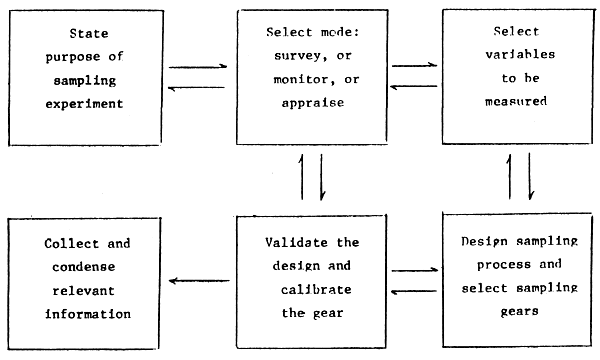
Figure 1 Major components of a sampling experiment. Two arrows imply that a decision is normally reached iteratively after considering various alternatives
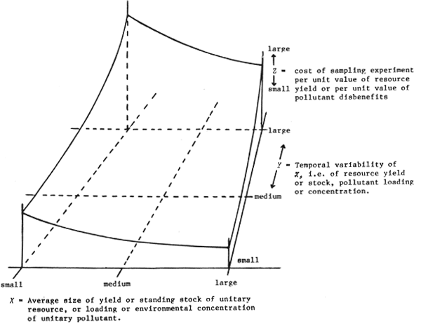
Figure 2 Sketch of the relative costs of a sampling experiment as a function of average value through time of benefits and/or disbenefits and temporal variability of those benefits and/or disbenefits. A basic assumption is that -- regardless of X and Y realities -- an experiment must produce estimates that meet a standard level of precision
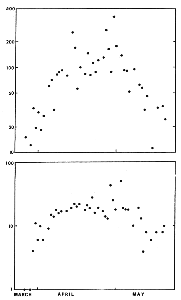
Figure 3 Top panel, kg of walleye per lift of trapnet during the spawning season. Bottom panel, percent of the walleye catch contributed by large, jumbo walleye. Vertical scales are logarithmic. (Data from a commercial fishery in southwestern Lake Erie, courtesy of Mr. M. Hosko)
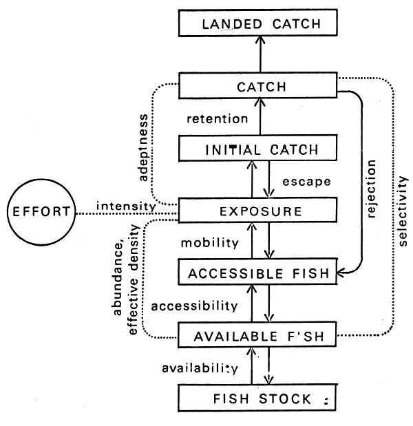
Figure 4 A model of the capture process that illustrates the meaning of various terms commonly used in discussing sampling methods (Hamley, 1974). Another term, catchability, is often used to relate catch to the fish stock assuming full availability and accessibility
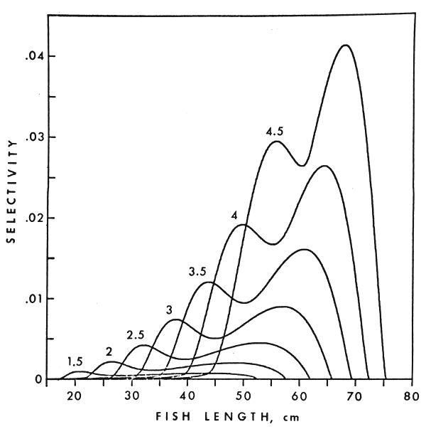
Figure 5 Selectivity of gill nets to walleye. Particulars on gill nets, habitat, sampling season, etc., are as given by Hamely and Regier (1973)