![]()
![]()
![]()
by
RICHARD J. BERRY and KENNETH N. BAXTER
Bureau of Commercial Fisheries Biological Laboratory
Galveston, Texas 77550, U.S.A.
Abstract
Studies of the feasibility of predicting the size of annual crops of brown shrimp (Penaeus aztecus) have been underway since the early sixties at the Bureau of Commercial Fisheries Biological Laboratory, Galveston, Texas. They are based on the premise that the relative abundance of postlarval or juvenile shrimp is indicative of subsequent commercial supplies. The present paper reviews the development of these studies, discusses sampling problems in measuring postlarval abundance, and correlates abundance indices between life history stages. Analyses of landing statistics indicate that predictions of brown shrimp abundance may be applicable to broad geographic areas of the Gulf of Mexico.
PREVISION DE L'ABONDANCE DES CREVETTES Penaeus aztecus DANS LE NORD-OUEST DU GOLFE DU MEXIQUE
Résumé
Depuis le début des années 60, le Laboratoire de biologie du Bureau des pêches commerciales de Galveston (Texas) étudie la possibilité de prévoir l'ampleur des captures annuelles de Penaeus aztecus, en se fondant sur l'hypothèse selon laquelle l'abondance relative des stades postlarvaires ou juvéniles de cette crevette fournit un indice des disponibilités ultérieures pour la pêche commerciale. La communication traite des progrès réalisés au cours de ces études, examine les problèmes d'échantillonnage associés à la mesure de l'abondance des postlarves, et met en corrélation les indices d'abondance à divers stades du cycle biologique. L'analyse des statistiques des apports fait penser que les méthodes de prévision de l'abondance de P. aztecus pourraient valoir pour de larges zones géographiques du golfe du Mexique.
PRONOSTICO SOBRE LA ABUNDANCIA DE PENAEUS AZTECUS AL NOROESTE DEL GOLFO DE MEXICO
Extracto
En el Laboratorio Biológico de la Oficina de Pesca Comercial de Galveston, Texas, se han llevado a cabo desde principios de 1960 investigaciones para averiguar la posibilidad de predecir la magnitud de las cosechas de camarón marrón (Penaeus azteous). Tales estudios se basan en el supuesto de que la abundancia relativa de camarón, en su fase postlarval o juvenil constituye un índice de las posteriores disponibilidades comerciales. En este ensayo se examina el desarrollo de estos estudios, se discuten los problemas de muestreo que implica la medición de la abundancia de ejemplares en fase postlarval y se ponen en relación los índices de abundancia entre las distintas fases del ciclo vital. Los análisis de las estadísticas de desembarque indican que los pronósticos sobre la abundancia de camarón marrón se pueden aplicar a amplias zonas geográficas del Golfo de México.
Biologists at the Bureau of Commercial Fisheries Biological Laboratory, Galveston, Texas began studies in the early sixties to investigate possibilities of predicting the annual abundance of brown shrimp (Penaeus aztecus Ives). This work was based on the premise that the number of postlarval shrimp collected during their movement from the Gulf to coastal bays and the density of juvenile shrimp in estuarine areas bear a proportional relation to subsequent commercial supplies. Several other groups of biologists, working under contract with our laboratory or independently, have pursued the same approach along various parts of the Gulf and south Atlantic coasts. A sizable number of general references to these studies have appeared in annual reports of the laboratory at Galveston, in Commercial Fisheries Review and in Louisiana Conservationist. More detailed reports include those of Baxter (1963), Baxter and Renfro (1967), Christmas, Gunter and Musgrave (1966), Louisiana Wild Life and Fisheries Commission (1964), St. Amant, Corkum and Broom (1963), and St. Amant, Broom and Ford (1966).
The present paper provides a review of studies on shrimp prediction underway at the Biological Laboratory in Galveston. It demonstrates the possibilities and limitations of current approaches to the problem so that others may benefit from our experiences.
Possible approaches to predicting shrimp abundance are limited because little is known about factors that influence the size of the populations. Without this information, we can seek a correlation only between measures of abundance at two life history stages and base predictions on the earlier measure. Fortunately, brown shrimp pass through reasonably distinct stages and it is possible to follow the development of a brood for several months. Spawning takes place in offshore oceanic waters and the young shrimp enter estuaries as postlarvae. After a period of rapid growth to a total length (tip of rostrum to end of telson) of 50 to 120 mm, they return offshore to depths of 30 to 80 m. The shrimp are fished commercially during both the estuarine and oceanic portions of their life if local conditions and statutes permit.
2.1 Postlarvae
A small-scale study to investigate seasonal changes in the movement of postlarval shrimp through the principal entrance to Galveston Bay began in November 1959 as part of an expanding shrimp research program. Collections of organisms near the shoreline of the entrance were made twice each week with the 1.5-m hand-drawn beam trawl described by Renfro (1963). Tows were made alternately in the morning and afternoon in an effort to sample during both ebb and flood tides each week. Penaeid shrimp were separated from the catch, identified, and counted at the laboratory. Details of sampling procedures and species identification were provided by Baxter (1963) and Baxter and Renfro (1967). Sampling was interrupted in May 1961 because of the pressing needs of other projects.
The significance of the catch data on postlarvae gathered between November 1959 and May 1961 became apparent shortly after sampling was suspended. Comparatively high numbers of postlarvae were caught in the early spring of 1960 and were followed by near record catches of brown shrimp in the commercial fishery during summer months. In 1961, our catches of postlarvae were small as were later commercial harvests, suggesting that catch data on postlarvae were indicative of brown shrimp abundance.
Semiweekly sampling for postlarvae was resumed in August 1961 with a new objective - to investigate the feasibility of predicting the relative abundance of commercial shrimp from catches of postlarvae. Sampling procedures were not changed because we anticipated that a simple and inexpensive technique for predicting would be more acceptable to agencies responsible for shrimp management than would complex sampling schemes. With the exception of a brief interruption caused by Hurricane Carla in September 1961, a routine schedule of sampling has been followed to the present. The location of the four stations at which collections were obtained is shown in Fig. 1.
2.2 Juvenile shrimp
Within 6 to 12 weeks after they enter estuaries, young shrimp grow to a size (70 to 100 mm in total length) that is favored by sport fishermen as bait. A seasonal bait shrimp fishery has developed in Galveston Bay during recent years to supply this market. Shrimp are harvested with otter trawls towed by skiffs or small trawlers and then distributed to dealers who sell them to sport fishermen (Inglis and Chin, 1966).
A continuing survey of the bait shrimp fishery of Galveston Bay began in 1957; its early results, including data on landings and species composition, were reported by Chin (1960). Since June 1959, statistics of fishing effort also have been gathered on a weekly schedule. The survey procedure requires that interviews be obtained from at least half of the bait shrimp dealers and fishermen in the bay area each week, and a visual check is made of other bait shrimp stands to determine how many are open for business. From this information, total landings and fishing effort are estimated. Species and size composition of landings are assessed from samples of shrimp purchased weekly from a random selection of dealers.
2.3 Adult shrimp
All shrimp landed by the commercial fishery and sold for human consumption are here classed as adults, whereas those taken by the bait fishery are considered to be juveniles. This distinction is based on the source of landing data rather than the stage of maturity of the shrimp. The classification is valid as it pertains to bait shrimp but is arbitrary as applied to commercial landings. The latter consist of a large range of sizes that by Renfro's (1964) definitions would be classed as juvenile, subadult, and adult shrimp.
Landing data for the commercial fishery are available in monthly tabulations published by the Fish and Wildlife Service in the Current Fishery Statistics series under the title Gulf Coast Shrimp Data. A description of these tabulations and of survey procedures used in gathering the data was given by Kutkuhn (1962). Data are grouped according to species and size composition of landings as well as depth and location from which catches originate. The geographic areas and coded subareas to which information on catches is assigned as it is obtained are outlined in Fig. 2. The data of interest in the present study are those pertaining to subarea 18 and adjacent inshore waters of Galveston Bay.
Predictions of the relative size of adult shrimp stocks from samples of postlarvae or juveniles require an index of abundance at these life history stages and definitions of the relation between indices. The reliability of forecasts will depend on the accuracy and precision of the measures of abundance, provided that mortalities between stages do not depart greatly from the average.
3.1 Postlarvae
3.1.1 Postlarvae of significance to later harvests Our data, in the form of postlarval catches, bait shrimp landings and commercial harvests, indicate that the bulk of the brown shrimp crop develops from postlarvae that enter estuaries between early February and the end of May. Attempts to identify more exactly the group of postlarvae that best indicates later harvests are hampered, however, by seasonal and annual variation among our sample data. Counts of brown shrimp postlarvae from each collection made from February through May of 1960–66 are listed in Table I. Catches made in 1960 and 1961 appear to vary more among collection dates than those of later years, but part of the variation may have resulted from the change in location of the sampling site (from station 1 to station 2) in the latter part of 1961 (Fig. 1).
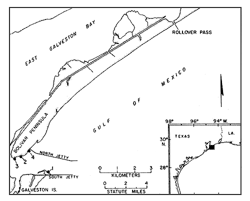
Fig. 1 Locations of stations at which postlarval shrimp have been collected on a routine basis (after Baxter, 1963). Periods during which samples were taken at the different stations were: station 1, November 1959–September 1961; station 2, September 1961–November 1961; station 3, June and July 1962; and station 4, November 1961 to date.
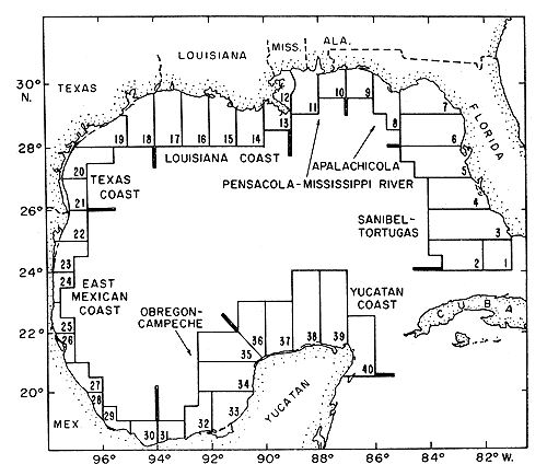
Fig. 2 Geographic areas and subareas in the Gulf of Mexico used to identify the origin of shrimp landings (after Kutkuhn, 1962).
TABLE I
Counts of postlarval brown shrimp caught in semiweekly collections in February, March, April and May, 1960–66
| Month | 1960 | 1961 | 1962 | 1963 | 1964 | 1965 | 1966 |
| February | 1 | 0 | 1 | 0 | 0 | 51 | 0 |
| 0 | 0 | 73 | 0 | 2 | 16 | 0 | |
| 2 | 0 | 34 | 0 | 0 | 16 | 4 | |
| 0 | 1 | 196 | 0 | 14 | 143 | 5 | |
| 3 | 4 | 48 | 0 | 3 | 142 | 591 | |
| 3 | 0 | 222 | 0 | 0 | 249 | 3 | |
| 2 | 0 | 53 | 0 | 0 | 120 | 22 | |
| 2 | 1 | 1,220 | 0 | 0 | 77 | 57 | |
| March | 0 | 6 | 0 | 441 | 0 | 24 | 32 |
| 0 | 5 | 40 | 16 | 3 | 13 | 51 | |
| 6 | 2 | 368 | 288 | 26 | 50 | 526 | |
| 53 | 1 | 66 | 21 | 46 | 612 | 83 | |
| 39 | 97 | 8 | 280 | 215 | 198 | 427 | |
| 72 | 28 | 506 | 286 | 765 | 30 | 117 | |
| 39 | 1 | 526 | 986 | 246 | 416 | 312 | |
| 1 | 2 | 140 | 114 | 110 | 38 | 206 | |
| 4,710 | 42 | 75 | 2 | 583 | 136 | 67 | |
| April | 3,680 | 6 | 1,682 | 360 | 399 | 193 | 107 |
| 86 | 12 | 234 | 3,521 | 383 | 48 | 369 | |
| 5 | 4 | 24 | 147 | 117 | 498 | 434 | |
| 1,000 | 1 | 135 | 54 | 432 | 187 | 749 | |
| 100 | 209 | 192 | 167 | 160 | 250 | 423 | |
| 9 | 10 | 44 | 44 | 38 | 205 | 264 | |
| 50 | 3 | 103 | 103 | 8 | 105 | 116 | |
| 56 | 2 | 3 | 93 | 64 | 142 | 24 | |
| 3 | 2 | 2 | 41 | 2 | 313 | 40 | |
| May | 0 | 51 | 4 | 68 | 58 | 88 | 84 |
| 4 | 1 | 250 | 181 | 294 | 67 | 24 | |
| 6 | 889 | 23 | 71 | 60 | 178 | 8 | |
| 1 | 1 | 7 | 10 | 19 | 160 | 2 | |
| 2 | 1 | 2 | 16 | 31 | 213 | 18 | |
| 9 | 1 | 0 | 17 | 579 | 39 | 8 | |
| 7 | 1 | 0 | 134 | 4 | 47 | 10 | |
| 5 | 1 | 0 | 29 | 89 | 212 | 11 | |
| 0 | 1 | 3 | 28 | 9 | 2 | 1 |
1 Scheduled sample not taken
2 No entry because of 4-week month
In most years, the largest numbers of postlarvae were taken in March and April, but abundance within these months seems to follow no regular trend. Collections made in February differ considerably from year to year, ranging from no postlarvae to relatively large numbers. Those from May appear to reflect a decline from the March-April peak, but differences between years are great. Because of the lack of a consistent pattern in these data, our decision on samples to include in an index had to be largely subjective.
3.1.2 Sampling variability Barnes (1952) and others have shown that counts from catches of marine organisms do not necessarily conform to a normal distribution and that the original data often must be transformed before standard statistical tests are employed. A proportional relation between the standard deviation and the mean of sample catches indicates that a logarithmic transformation is appropriate (Fig. 3). The transformation eliminates the relation (Fig. 3) and causes this type of data to follow a normal distribution more closely (Fig. 4). More meaningful estimates of the sample mean or variance can be obtained from transformed data than from the original sample counts. For this reason, our counts of postlarvae were converted to logarithms before analysis and sample averages are reported as geometrio rather than arithmetic means.
Special studies were started in the spring of 1963 to investigate the influence of several potential sources of sampling variability. In particular, we wanted to determine the reliability of our sampling gear, the effects of tides on postlarval catches, and the possibility of diel differences in the availability of postlarvae to our net. From March through August, three samples rather than one were taken on regular semiweekly collection dates. Also, three concurrent samples were obtained at 2-h intervals over a 4-day period in early April. These two sets of data, each consisting of 48 replicated observations, provided considerable insight into the sampling problems.
The results of an analysis of variance of each set of replicated samples (Tables II and III) constitute tests of the performance of the beam trawl. Variations between sampling times was significantly greater than between replicates. Results were surprisingly similar for the two groups of data and, for each set, only 2 percent of the total variation was due to differences among replicates. This information assured us that the beam trawl provides a satisfactory sample in the postlarvae present in the vicinity of our sampling site. It also showed that the total variation of samples taken over a period of 4 days was almost as great as that from collections made during 6 months - a result of the fact that the range in numbers of postlarvae at a given location can change from zero to several thousand within a few hours.
TABLE II
Analysis of variance of replicated samples of postlarvae caught at 2-hour intervals over a 4-day period
| Source of variation | Degrees of freedom | Sum of squares | Mean square | F |
| Between times | 47 | 39.9914 | 0.8509 | 76.7 |
| Between replicates | 96 | 1.0666 | 0.0111 | Table value at the 0.01 level = 1.73 |
| Total | 143 | 41.0580 |
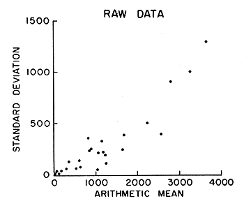
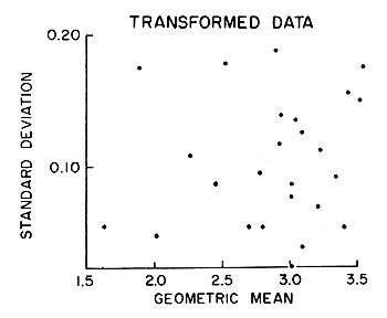
Fig. 3 Relation between the standard deviation and the mean of a selected group of postlarval shrimp catches made in 1963.
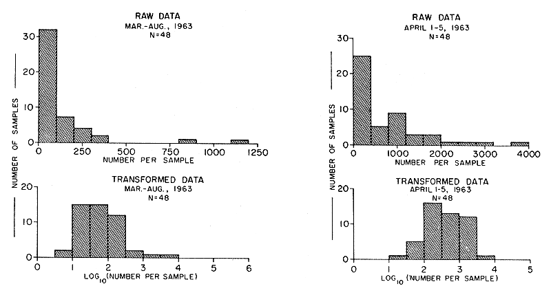
Fig. 4 Frequency distributions of numbers of postlarvae in samples (N) illustrating an effect of the logarithmic transformation. One catch was too large (3,286) to be shown in the upper left-hand graph.
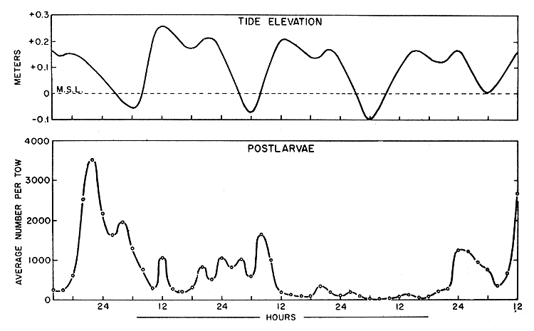
Fig. 5 Catches of postlarvae and tide elevation at the regular sampling site in the entrance to Galveston Bay, 1–5 April 1963.
TABLE III
Analysis of variance of replicated samples of postlarvae caught at 3-to 5-day intervals over a 6-month period
| Source of variation | Degrees of freedom | Sum of squares | Mean square | F |
| Between times | 47 | 48.4585 | 1.0310 | 44.7 |
| Between replicates | 96 | 2.2156 | 0.0231 | Table value at the 0.01 level = 1.73 |
| Total | 143 | 50.6741 |
The collections made at 2-h intervals in April 1963 provided no obvious answers to questions concerning the effects of tides or diel differences in the availability of postlarvae (Fig. 5). Similar collections made at the same site in March 1964 also showed no apparent correlations. We concluded that our sampling station was probably in a position where water movements differed from recorded tide levels. To pursue the problem further, we made hourly collections of postlarvae and measurements of water movements over two 3-day periods in the spring of 1965 at Rollover Pass, a narrow, secondary inlet to Galveston Bay (see Fig. 1). Because of fast water currents at this pass, samples were taken with a 0.5-m plankton net suspended from a bridge rather than with the beam trawl. The number of postlarvae caught varied with water movements, at least when currents were strong (Fig. 6). Presumably, specimens caught during ebb tides were those that had been carried into the bay on a previcus flood tide. If postlarvae are also transported through the principal entrance to Galveston Bay by water currents, it follows that any of a number of conditions that affect the direction and velocity of the flow of water can likewise influence the numbers of postlarvae carried past our sampling station. Included among these conditions may be normal tidal changes, storms with their accompanying wind-driven water movements, and excessive amounts of runoff from land.
3.1.3 Indices of abundance The number of combinations of data that might be used to calculate an abundance index for postlarvae is almost unlimited. Baxter (1963) used the arithmetic mean of the number of brown shrimp postlarvae in collections made from February through May. Christmas, Gunter and Musgrave (1966), who made their observations in Mississippi Sound, used the average catch of postlarval brown shrimp taken from February through July. The most appropriate method of combining data on postlarvae to form an index is open to question. The decision should be based on knowledge of the sampling distribution of counts of postlarvae, but our data are not sufficient to permit a definite choice. Conceivably, the distribution of numbers of postlarvae per sample might form a normal curve if enough collections were made during periods of peak abundance. If so, an index should be formed from an arithmetic mean. The small number of our collections make it advisable to transform counts of postlarvae to logarithms in order that they will approximate a normal curve. A geometric mean is then appropriate for an index number. It should be emphasized, however, that the method of combining data to form an index is much less important than the quality of data included.
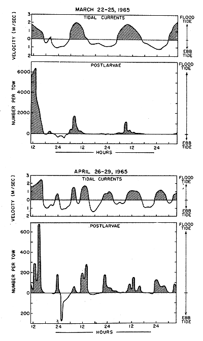 | 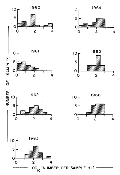 | ||
| Fig. 6 | Relation of catches of postlarvae to tidal currents at Rollover Pass, a relatively narrow inlet to Galveston Bay. Shaded areas indicate water or postlarvae moving into the bay. | Fig. 7 | Distributions of counts of brown shrimp postlarvae collected in March and April 1960–66. |
Distributions of counts of postlarvae collected in March and April 1960–66 are presented in Fig. 7. Collections represented in this figure and listed in Table I are those from which we might logically expect to develop an index to the commercial stock of brown shrimp making its appearance in July and August. The shapes or midpoints of these distributions change little if samples from February or May are included. Without resorting to calculations, it is evident that the means of the distribution are fairly similar for all years except 1961. This uniformity implies that postlarval brown shrimp stocks were of the same general magnitude in most of these years - a situation that is not supported by data from the bait and commercial fisheries.
A series of geometric and arithmetic index numbers are provided in Table IV. Also listed, for comparison, are estimates of the relative size of brown shrimp stocks in Galveston Bay in the early summers of 1960–66. The latter were derived from data on bait shrimp landings and are discussed in more detail in a subsequent section. In general, poor correlations exist between the indices of abundance of postlarvae and bait shrimp. We have greater confidence in the indices based on bait shrimp catches and believe that reliable measures of postlarvae will require changes in past sampling procedures.
TABLE IV
Index numbers (average number per sample) based on catches of brown shrimp postlarvae in the spring months of 1960–66
| Indices | 1960 | 1961 | 1962 | 1963 | 1964 | 1965 | 1966 |
| Geometric means | |||||||
March-April | 41 | 9 | 77 | 152 | 82 | 120 | 155 |
March-May | 17 | 14 | 30 | 96 | 68 | 115 | 64 |
February-May | 11 | 6 | 37 | 32 | 29 | 103 | 41 |
| Arithmetic means | |||||||
March-April | 583 | 29 | 250 | 410 | 211 | 192 | 242 |
March-May | 382 | 81 | 174 | 287 | 182 | 172 | 167 |
February-May | 293 | 57 | 188 | 219 | 140 | 155 | 148 |
| Best estimate of relative population size1 | 56 | 26 | 29 | 37 | 27 | 42 | 192 |
1 Based on catch per unit of effort by the Galveston Bay bait shrimp fishery, 25 April – 31 July.
2 We believe that this estimate is biased and that it should have been about 32.
3.1.4 Plans for the future Experience to date has identified several sources of variation that can affect an index of postlarval abundance and provides a base from which to plan future investigations. An apparent shortcoming of past data is the small number of samples obtained during period of peak postlarval movements. We are considering three ways of increasing the frequency of sampling and thereby reducing the variability of an index:
Collect postlarvae by present methods, but increase the number of collections by a factor of at least 5, or preferably, 10. This change would give 10 or 20 samples each week during periods when peak numbers of brown shrimp are entering Galveston Bay. If a new station were located where the relation between the numbers of postlarvae in samples and tidal movements is clear-cut fewer samples might suffice. The expense of this approach in terms of the time and manpower needed for sampling could easily become prohibitive, however.
Attempt to minimize the influence of environmental variables, especially tidal influences, on catches by establishing a collection site seaward of the entrance to the bay. Although fewer samples might be required, the cost per sample would increase and new sampling techniques would have to be developed.
Install a mechanical sampling device that takes small samples at frequent intervals or continuously at a convenient location in the entrance to the bay. The advantage gained by continuous sampling is that a large proportion, essentially all, of the variation caused by environmental factors can be considered as random. If the device were placed in a location where a nearly constant proportion of the entering postlarval shrimp passes, the reliability of an index would depend principally on the efficiency of the gear.
The feasibility of investing money in the development and maintenance of more expensive sampling gear depends on the ultimate value of predictions. It is impossible to estimate their worth because we have no way of judging how they might affect operations of the fishery. Presumably, advance information regarding shrimp abundance would enable various elements of the shrimp industry to reduce costs and perhaps divert efforts when poor harvests are expected or to expand facilities and clear distribution channels for good harvests. The benefits of these procedures would be relatively small in their application to the fishery in the Galveston area, but could be substantial if applied to the entire Gulf of Mexico shrimp industry and its supporting services. Relatively few postlarval sampling stations might serve wide areas of the Gulf because trends in the abundance of a species of shrimp may be similar over wide geographic areas. This consistency in trends is explored further in a later section.
3.2 Juvenile shrimp
The relative size of shrimp stocks in Galveston Bay is reflected better by landings of the bait shrimp fishery than by our catches of postlarvae. This fishery yields information that otherwise could be obtained only through an extensive and costly program of field sampling. As suggested by the home locations of bait shrimp dealers and boats in Fig. 8, the operations of the fishery cover most peripheral areas of Galveston Bay.
Time is important when we consider predicting the size of commercial stocks from statistics of the bait fishery. Brown shrimp are most abundant in bait landings from Galveston Bay during May, June, and July. Offshore commercial fishing for young-of-the-year brown shrimp begins in late June and reaches peak intensity in July or August. Useful predictions must be based on early season catch data from the bait fishery.
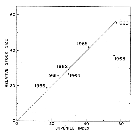
The brown shrimp stock of principal interest for predictions may be defined as that represented by bait fishery landings from 25 April to 31 July. These dates are arbitrary but cover most of each year's brown shrimp stock in the bay and probably include most of the shrimp that appear as postlarvae in March, April, and May. The earliest catches of brown shrimp by the bait fishery are expected about 25 April, and the species is no longer abundant in the bay after 31 July. Estimates of the average catch of brown shrimp per hour of fishing each week from 25 April to 31 July are shown in Fig. 9 for each year of our study. The original data were gathered by weekly periods, but minor adjustments were necessary to make the dates correspond among years in this figure. By summing weekly estimates of catch per effort for a season and dividing by the number of weeks (14), we obtain a single number proportional to the size of the brown shrimp stock in a given year. These figures must then be predicted from early season catch and effort data. The success of this approach depends on the similarity among years of the shape of the distribution of catch per effort at the same calendar periods. The formation of accumulative frequency distributions showed that the average catch per effort for the 14-week period could best be estimated from the average catch per effort from 25 April to 12 June. A close similarity exists between the early and full season measures of abundance in 6 of the 7 years, but not in 1963 (Fig. 10). Reference to Fig. 9 makes it apparent that in 1963 the stock of brown shrimp developed and moved out of range of the bait fishery earlier than usual.
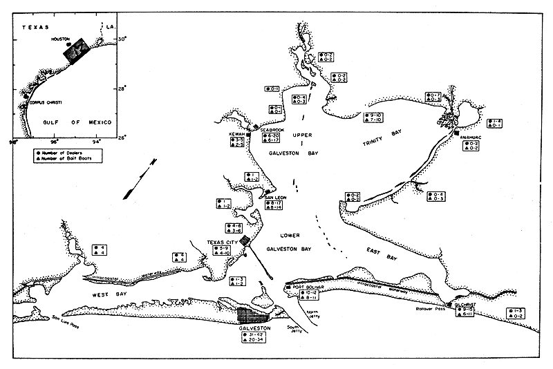
Fig. 8 Locations of bait dealers and bait boats in the Galveston Bay area, 1959–64.
On the basis of the positive relation between the growth of young brown shrimp and water temperatures demonstrated by Zein-Eldin and Aldrich (1965), it is reasonable to expect that unusually warm water influenced the early development of shrimp in 1963. Although water temperature data are not available, average air temperatures were above normal during March, April, and May 1963 (Table V). In fact, the average air temperature for April was the highest recorded in 1930–66.
TABLE V
Average monthly air temperatures (° C.) at the Galveston
Post Office Building for March, April, and May 1960–66
(Original data reported in ° F.)
| Month | 1960 | 1961 | 1962 | 1963 | 1964 | 1965 | 1966 | 91-year average |
| March | 13.8 | 18.2 | 15.7 | 17.8 | 15.5 | 13.9 | 15.9 | 16.7 |
| April | 20.4 | 19.1 | 20.2 | 22.5 | 20.8 | 21.7 | 20.5 | 20.6 |
| May | 23.1 | 23.9 | 24.7 | 25.1 | 24.9 | 24.6 | 24.0 | 24.3 |
| Average | 19.1 | 20.4 | 20.2 | 21.8 | 20.4 | 20.1 | 20.1 | 20.5 |
Source: Local Climatological Data, Galveston, Texas. Weather Bureau, U.S. Department of Commerce.
3.3 Adult shrimp
Landing and effort statistics, recorded monthly in Gulf Coast Shrimp Data, provide the information required to measure the abundance of adult shrimp. Indices for adult brown shrimp were calculated as the average catch per hour in July, August, and September in offshore waters, as reflected by interviews. Possible biases in these data, caused by variations in the size of fishing vessels and from inclusion of fishing effort directed toward other species, were avoided by selecting the information used. To reduce the quantity of data from landings made by small, inshore vessels, only catches from depths greater than 20 m were incorporated into indices. Also, data were not used if species other than brown shrimp made up more than an incidental portion of landings.
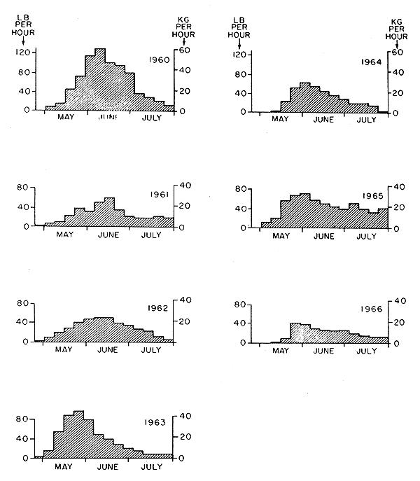
Fig. 9 Catch of brown shrimp per unit of fishing effort by the bait shrimp fishery in Galveston Bay, by weeks, from 25 April through 31 July, 1960–66.
 |  | ||
| Fig. 10 | The relation of the relative size of brown shrimp stocks from Galveston Bay (lb/h from 25 April to 31 July) and the index of juvenile brown shrimp abundance (lb/h from 25 April to 12 June). The equation Y = bx was used to fit the line to observations (other than that for 1963) because the intercept of the line derived from Y = a + bx did not differ significantly from zero. | Fig. 11 | The relation of the index to abundance of adult brown shrimp from subarea 18 (lb/h landed by the commercial fishery, July-September) and the relative size of stocks from Galveston Bay (lb/h landed by the bait shrimp fishery. 25 April to 31 July) for the years 1960–66. The equation Y = bx was used to fit the line to observations (other than that for 1966) because the intercept of the line derived from Y = a + bx did not differ significantly from zero. |
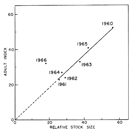
3.3.1 Indices for adult shrimp from Galveston Bay Landing and effort data from subarea 18 (Fig. 2) were used to derive indices for brown shrimp that presumably had moved offshore from the Galveston Bay system. Numerical values for these indices are listed in Table VI along with indices of abundance of juvenile shrimp and estimates of the relative size of stocks in the bay each year from 1960 to 1966. To repeat the definitions of indices derived for bay populations: relative stock size is the average of weekly estimates of the weight of brown shrimp caught per hour by the bait shrimp fishery in Galveston Bay from 25 April through 31 July, and the juvenile index is formed by the same means from bait fishery data collected from 25 April through 12 June. Since these two measures differ little from each other for 6 of the 7 years tested (Fig. 10), it may be possible to predict relative stock size in the bay by 12 June in most years. A similar correlation exists between relative stock size and the index for adult brown shrimp in offshore waters of subarea 18 (Fig. 11). In this graph, the point for 1966 does not fall on the trend line, but those for other years are reasonably close to it.
TABLE VI
Abundance indices for juvenile and adult brown shrimp and the relative size of stocks originating from Galveston Bay in 1960–66
| Measure of abundance | 1960 | 1961 | 1962 | 1963 | 1964 | 1965 | 1966 |
| Juvenile index | 57 | 24 | 30 | 561 | 29 | 41 | 182 |
| Relative stock size | 56 | 26 | 29 | 37 | 27 | 42 | 192 |
| Adult index | 52 | 23 | 24 | 33 | 27 | 41 | 322 |
1 The high index for juvenile brown shrimp in 1963 resulted from the unusually early emigration of shrimp from Galveston Bay
2 The lack of agreement between measures in 1966 cannot be explained with certainty. Possible causes are discussed in the text
We can only speculate why the data for 1966 did not follow the trend established for other years. Either the adult index overestimated the crop of brown shrimp in offshore waters or the measure of stock size for juvenile shrimp in Galveston Bay underestimated their abundance. The index for adult brown shrimp may have been influenced by entry into the fishery of several new vessels that fish two, 16-to 21-m nets rather than the usual pair of 14-m nets. On the other hand, unusual environmental conditions within Galveston Bay may have affected catches in the bait shrimp fishery. Abnormally large quantities of fresh water from spring floods that decreased the salinity of bay waters in May 1966 (Table VII) may have caused young shrimp to move seaward before they normally would do so. Measurements of total lengths of juvenile brown shrimp caught at the entrance to Galveston Bay averaged 49 mm on 11 May (Trent, personal communication) and 58 mm on 18 May (Trent, 1967). These shrimp were considerably smaller than those collected by Trent on later dates. Conceivably, part of the stock normally fished by the bait fishery moved beyond its reach and depressed abundance indices based on catches in the bay.
A final correlation, and the one of principal interest from the viewpoint of predictions, can be made between the indices for juvenile and adult brown shrimp. We have not portrayed these data in a graph because the relation between them is evident from the values listed in Table VI. The two measures are similar in 5 of the 7 years, but not in 1963 or 1966. With the exception of these 2 years, it would have been possible to predict the average fishing success (catch per hour) for offshore brown shrimp in July, August and September as early as 12 June.
TABLE VII
Measurements of the volume (million m3) of fresh water carried into Galveston Bay by the Trinity River during the spring, 1963–66
Month | 1963 | 1964 | 1965 | 1966 |
March | 137 | 286 | 604 | 192 |
April | 206 | 288 | 483 | 729 |
May | 583 | 216 | 1,441 | 3,943 |
June | 195 | 147 | 1,052 | 858 |
Source: Water Resources Division, U.S. Geological Survey, Austin, Texas
3.3.2 Indices for other areas of the Gulf We have calculated index numbers for brown shrimp in the offshore waters of subareas 11 and 13 through 21 (see Fig. 2 for locations) for those years for which interview information is available (Table VIII). These numbers, which represent the average weight of brown shrimp landed per hour of fishing from July through September, indicate that the relative density of this species was more similar within than between years over the range of the fishery from Alabama to the Mexican border. This region supplied 75 to 90 percent of the total U.S. landings of Gulf brown shrimp.
We are confident that, in general, these indices provide a correct picture of the abundance of brown shrimp, but several possible sources of error limit the value of comparisons among individual index numbers. The proportion of interviews obtained from vessel captains varies within and between subareas and seasons. Likewise, the depths in which fishing intensity is greatest, and consequently, the average size of shrimp caught, differs within and between regions and months. Because of these short-comings in the basic data, statistical analyses would add little to our interpretations of the index numbers. We can, however, help to substantiate differences between years by reference to landings from sections of the Gulf coast. A comparison of average index numbers and total annual harvests from Louisiana and Texas waters for 1958–65 shows that when total fishing effort remains at about the same level, as it did in these years, the indices provide good indications of total harvest (Fig. 12).
It is tempting to speak of predicting the relative abundance of brown shrimp along all of the Texas coast or over the entire northwestern portion of the Gulf of Mexico from estimates obtained from the bait fishery of Galveston Bay. Despite the strong correlations existing among these measures, we believe that predictions for such a broad area should be based on data from more than one sampling location.
Certain generalizations are justified on the basis of evidence presented concerning so-called good and poor years for brown shrimp:
Predictions of size of brown shrimp stocks in the Gulf of Mexico may require information (concerning the relative abundance of postlarvae or juveniles) from a relatively small number of judiciously selected sampling sites.
Of the many factors that influence the size of brown shrimp populations, only those that affect broad areas of the Gulf have a major effect on abundance. This implies that current fishing practices, such as differences in the time and intensity of fishing, or variations in laws regulating catches have little influence on population size, although they obviously affect harvests.
TABLE VIII
Indices to the abundance of adult brown shrimp (July-September) in subareas 11 and 13 through 21 for the years 1958–1965. Indices for each subarea are ranked between years to facilitate comparisons
| Subarea | 1958 | 1959 | 1960 | 1961 | 1962 | 1963 | 1964 | 1965 |
| 11 | ||||||||
Index | 25 | 37 | 36 | 19 | 17 | 31 | 32 | 35 |
Rank | 6 | 1 | 2 | 7 | 8 | 5 | 4 | 3 |
| 13 | ||||||||
Index | 27 | 32 | 38 | 19 | 22 | 31 | 20 | 35 |
Rank | 5 | 3 | 1 | 8 | 6 | 4 | 7 | 2 |
| 14 | ||||||||
Index | 26 | 42 | 37 | 24 | 21 | 38 | 22 | 48 |
Rank | 5 | 2 | 4 | 6 | 8 | 3 | 7 | 1 |
| 15 | ||||||||
Index | 28 | 33 | 37 | 22 | 18 | 33 | 25 | 29 |
Rank | 5 | 2.5 | 1 | 7 | 8 | 2.5 | 6 | 4 |
| 16 | ||||||||
Index | 36 | 41 | 44 | 21 | 17 | 41 | 26 | 38 |
Rank | 5 | 2.5 | 1 | 7 | 8 | 2.5 | 6 | 4 |
| 17 | ||||||||
Index | 32 | 50 | 65 | 25 | 21 | 34 | 27 | 38 |
Rank | 5 | 2 | 1 | 7 | 8 | 4 | 6 | 3 |
| 18 | ||||||||
Index | 33 | 49 | 52 | 23 | 24 | 33 | 27 | 41 |
Rank | 4.5 | 2 | 1 | 8 | 7 | 4.5 | 6 | 3 |
| 19 | ||||||||
Index | 33 | 44 | 45 | 22 | 21 | 33 | 25 | 36 |
Rank | 4.5 | 2 | 1 | 7 | 8 | 4.5 | 6 | 3 |
| 20 | ||||||||
Index | 27 | 49 | 45 | 25 | 26 | 35 | 28 | 39 |
Rank | 6 | 1 | 2 | 8 | 7 | 4 | 5 | 3 |
| 21 | ||||||||
Index | 27 | 46 | 41 | 28 | 25 | 33 | 24 | 34 |
Rank | 6 | 1 | 2 | 5 | 7 | 4 | 8 | 3 |
| Average | ||||||||
Index | 29 | 42 | 44 | 23 | 21 | 34 | 26 | 37 |
Rank | 5 | 2 | 1 | 7 | 8 | 4 | 6 | 3 |
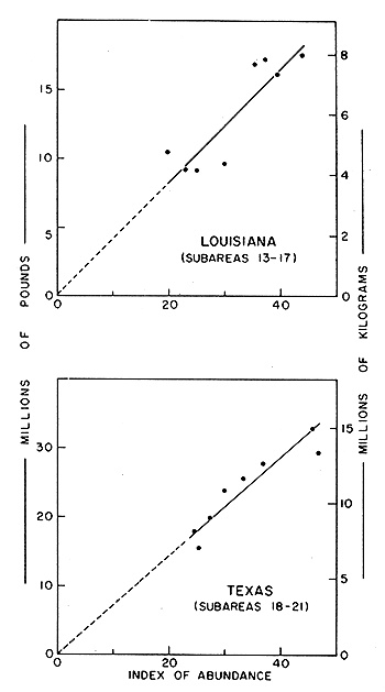
Fig. 12 The relation of annual landings and average indices of abundance of adult brown shrimp along the Louisiana and Texas coasts, 1958–65.
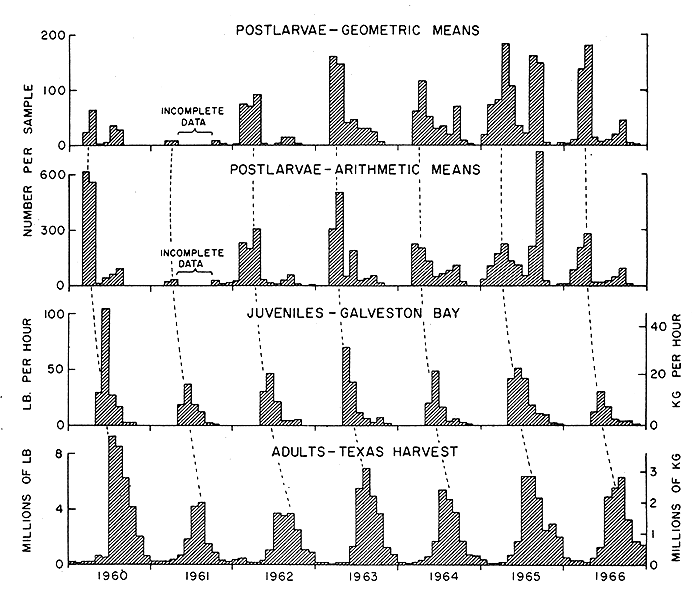
Fig. 13 Abundance of brown shrimp at the postlarval, juvenile and adult stages by months, 1960–66.
We have emphasized problems in sampling postlarvae and the interpretation of postlarval counts. These topics assume major importance when one speaks of the statistical significance of an index number or the reliability of a prediction. At the present early stage of such studies, it is equally important to recognize that collections of postlarvae can be used to advantage, even though forecasts must be of a very general nature.
The relation between our catches of postlarvae and the later abundance of juvenile and adult brown shrimp is shown in Fig. 13 for 1960–66. Again, postlarval abundance is portrayed in terms of both the arithmetic and geometric averages of monthly counts. Adult abundance is shown as monthly landings of brown shrimp from the Texas coast.
Finally, we wish to make a distinction between forecasts of adult abundance based on postlarval and juvenile indices. Despite serious problems in the sampling of postlarvae, we believe that predictions based on postlarval indices have greater potential value to the shrimp industry than those made from catches of juvenile shrimp because the information is available 4 to 6 weeks sooner.
Barnes, H., 1952 The use of transformations in marine biological statistics. J. Cons. perm. int. Explor. Mer, 18(1):61–71
Baxter, K.N., 1963 Abundance of postlarval shrimp - one index of future fishing success. Proc. Gulf Caribb. Fish. Inst., 15(1962):79–87
Baxter, K.N. and W.C. Renfro, 1967 Seasonal occurrence and size distribution of postlarval brown and white shrimp near Galveston, Texas, with notes on species identification. Fishery Bull. Fish Wildl. Serv. U.S., 66(1):149–58
Chin, E., 1960 The bait fishery of Galveston Bay, Texas. Trans. Am. Fish. Soc., 89(2):135–41
Christmas, J.Y., G. Gunter and P. Musgrave, 1966 Studies of annual abundance of postlarval penaeid shrimp in the estuarine waters of Mississippi, as related to subsequent commercial catches. Gulf Res. Rep., 2(2):177–212
Inglis, A. and E. Chin, (revised by K.N. Baxter), 1966 The bait shrimp industry of the Gulf of Mexico. Fishery Leafl. Fish Wildl.Serv., U.S., (582):10 p. Also issued as Fishery Leafl. Fish Wildl. Serv., U.S., (480): 14 p. (1959)
Kutkuhn, J.H., 1962 Gulf of Mexico commercial shrimp populations - trends and characteristics 1956–59. Fishery Bull. Fish. Wildl. Serv., U.S., 62(212):343–402
Louisiana Wildlife and Fisheries Commission, 1964 Shrimp research. Bienn.Rep.La.Wildl. Fish. Commn, 10:161–73
Renfro, W.C., 1963 Small beam net for sampling postlarval shrimp. Fishery Research Biological Laboratory, Galveston. Circ. Fish Wildl.Serv., Wash., (161):86–7
Renfro, W.C., 1964 Life history stages of Gulf of Mexico brown shrimp. Fishery Research Biological Laboratory, Galveston. Circ. Fish Wildl. Serv., Wash., (183): 94–8
St. Amant, L.S., J.G. Broom and T.B. Ford, 1966 Studies of brown shrimp Penaeus aztecus, in Barataria Bay, Louisiana, 1962–1965. Proc. Gulf Caribb. Fish. Inst., 18:1–17
St. Amant, L.S., K.C. Corkum and J.G. Broom, 1963 Studies on growth dynamics of the brown shrimp, Penaeus aztecus, in Louisiana waters. Proc. Gulf Caribb. Fish. Inst., 15:14–26
Trent, L., 1967 Size of brown shrimp and time of emigration from the Galveston Bay system. Proc. Gulf Caribb. Fish Inst., 19:7–16
Zein-Eldin, Z.P. and D.V. Aldrich, 1965 Growth and survival of postlarval Penaeus aztecus under controlled conditions of temperature and salinity. Biol. Bull. mar. biol. Lab., Woods Hole, 129(1):199–216
Acknowledgements
Many associates have made significant contributions to the development and progress of these studies. We are particularly indebted to J.H. Kutkuhn and W.C. Renfro who initiated the work. M.J. Duronslet, C.H. Furr, Jr., C.J. Guice, C.E. Knight, F. Marullo, T.W. Turnipseed, and L.M. Wisepape collected and processed much of the postlarval and bait shrimp data.
![]()
![]()
![]()