C. Methods of Prognosis and Monitoring

Paper 8 - 1. Soil and hydrologic surveys for the prognosis and monitoring of salinity and alkalinity
Paper 9 - 2. Soils and hydrologic surveys
Paper 10 - 4. Use of satellite imagery for salinity appraisal in the Indus Plain
Paper 10 - 5. Laboratory and field characterization
Paper 15 - 6. Modelling of salt movement through the soil profile

Paper 8 - 1. Soil and hydrologic surveys for the prognosis and monitoring of salinity and alkalinity

by

I. Szabolcs, G. Varallyay and K. Darab
Research Institute for Soil Science and Agricultural Chemistry of the Hungarian Academy of Sciences
and
National Institute for Agricultural Quality Testing
Budapest

1. INTRODUCTION

The main cause of the formation and occurrence of salt affected soils is the accumulation of Na⁺ ions in the solid and/or liquid phases of the soil, i.e. the presence of dissolved sodium salts in the soil solution and/or exchangeable Na⁺ ions in the soil absorption complex. These two phenomena are directly or indirectly responsible for the low fertility of salt affected soils. The high salt concentration of the soil solution is directly toxic to plants in several cases, it limits their water and nutrient uptake, metabolism and results in physiological deteriorations. The high sodium saturation of the soil causes increased hydration, dispersion and peptization of soil colloids, structural destruction, aggregate failure and consequently results in unfavourable physical and hydrophysical properties (low available moisture range, high wilting percentage, swelling, low infiltration rate, low saturated and unsaturated hydraulic conductivity, etc.). All these factors limit the agricultural potential of salt affected areas and determine both the possibilities for their rational land use (including cropping pattern, agrotechnics, irrigation, etc.) and the necessity and optimum combination(s) of ameliorative measures (leaching, drainage, chemical amendments, etc.).

The final aim of any research and survey on salt affected soils is to establish the exact scientific basis for efficient salinity and alkalinity control including:

- amelioration of salt affected soils;
- regulation of actual salinity and alkalinity;
- prevention of salinization and alkalization processes, limiting their further development.

- to describe the salinization and alkalization and reverse processes exactly;

- to characterize the influencing factors and to analyse their mechanisms and relationships quantitatively;

- to elaborate a comprehensive prognosis system for the prediction of these processes;

- to establish a regular monitoring system for the continuous registration of salinity and alkalinity changes due to natural factors or human activity.

2. GENERAL CONSIDERATIONS ON PROGNOSIS AND MONITORING

For the description and prediction of salinization and alkalization processes the following factors have to be considered.

i. The main actual and potential sources of water soluble salts (especially sodium salts) have to be identified and quantitatively characterized (ground-waters; deep subsurface waters; irrigation waters; seepage waters from higher lands, irrigated areas, canals, reservoirs; inundation and runoff waters; salt water intrusion; deeper soil horizons, geological layers; products of local weathering; airborne salts; etc.).

ii. The main features of the salt regime have to be characterized (salt balances: spatial distribution, both vertical and horizontal, and seasonal dynamics of water soluble salts and mobile sodium compounds; solute movement in saturated and unsaturated soil layers; diffusion; solubility changes; interactions between the soil's solid, liquid and gaseous phases; etc.).

iii. The whole range of environmental factors influencing the role and importance of various salt sources and the components of the salt regime summarized above have to be analysed (meteorological, geographical, geological, geochemical, geomorphological, hydrogeological and hydrological conditions; topography; soil conditions: physical, hydrophysical, physico-chemical, chemical, biological soil properties and their spatial distribution, and seasonal dynamics, etc.).

iv. The impact of human activity (land use, agrotechnics, amelioration, irrigation, drainage, leaching, erosion control, water and soil pollution, etc.) has to be studied and accurately determined.

- preliminary (small or medium scale) reconnaissance survey and mapping;
- detailed (large scale) survey and mapping.

3. SMALL OR MEDIUM SCALE RECONNAISSANCE SOIL AND HYDROLOGICAL SURVEYS AND MAPPING

The aim of these surveys is to give a general outline of the actual salinity and alkalinity status in soils of a given area and of the potential possibilities of salinization and alkalinization and reverse processes. The reconnaissance type of low intensity surveys (scale 1:100 000, 1:200 000, 1:500 000 or similar) should not be limited to the project area but must be extended to the whole geographical unit (water catchment area, hydrological region, irrigation system, etc.). For these surveys all kinds of descriptive, numerical, cartographical and other materials (air photos, etc.) of meteorological observations, geomorphological, geological, hydrological and soil surveys can be used which give information on the factors summarized in the general considerations. The soil and hydrological surveys should cover the following factors:

A. Soil characteristics

i. general characteristics of the soil cover (associations of great soil groups and parent materials);

ii. general information on the dominant soil processes with an evaluation of the actual and potential soil forming factors;

iii. salinity and alkalinity status of soils (horizontal and vertical distribution, characteristic ion composition of soluble salts and their dynamics: general salt balances, soil reaction, exchangeable Na⁺ status) and potential factors of salinization and alkalization processes (hydrological conditions, salinity and alkalinity status of deeper soil horizons or geological layers, factorial salt balances).

B. Hydrological characteristics

i. groundwater conditions (depth and fluctuation of the water table, height of the water table above a reference level, horizontal flow of groundwater, sources of groundwater supply, concentration and chemical composition of the groundwater, evaluation of ground-water as a potential irrigation water, etc.);

ii. surface water conditions (concentration and chemical composition of surface water and its evaluation as potential irrigation water or as leaching water, hazards of waterlogging and flooding, hazard of seepage and salt water intrusion, etc.).

DS = S₂ - S₁ ..... (1)

DS = Salt or sodium balance: change of storage in the soil, t/ha
S₂ = Quantity of salts or mobile sodium at the end of the reference period, t/ha
S₁ = Quantity of salts or mobile sodium at the beginning of the reference period, t/ha

a. for the total salt content, or for various ions (when studying specific ion effects and chemical changes in the soil solution during filtration, etc.);

b. for the whole soil profile from the soil surface to the water table, or for various layers, horizons (when studying salt profile redistribution, hazard of resalinization, leaching efficiency, etc.) or for the root zone;

c. for soils, mapping units or territories (having a sufficiently homogeneous hydrological character);

d. for vegetation periods, irrigation seasons, seasons, years or longer periods of time (having a sufficiently homogeneous hydrological character).

The general equation of detailed (factorial) salt balances can be written, as follows:

DS = [P + I + R + G + W + F] - [1_p + 1_i + r + g + n] ..... (2)

DS = Salt balance

P = Quantity of salts derived from the atmosphere (airborne salts, rainfall, wind action, etc.)

I = Quantity of salts added with the irrigation water

R = Horizontal inflow of salts transported by surface waters (runoff, flood, waterlogging)

G = Horizontal inflow of salts transported by subsurface water (ground-waters, deep subsurface waters, etc.)

W = Quantity of salts derived from local weathering processes

F = Quantity of salts added with fertilizers and chemical amendments

1_p = Quantity of salts leached out by atmospheric precipitation

1_i = Quantity of salts leached out by irrigation (leaching) water

r = Horizontal outflow of salts (discharge) transported by surface waters

g = Horizontal outflow of salts transported by subsurface waters (drainage)

n = Quantity of salts taken up by plants and transported from the area with the yield

P, I, F and n can be measured and predicted easily; R and r can be estimated on the basis of topographical surveys, meteorological observations, surface water investigations and infiltration studies; G and g can be calculated from groundwater characteristics, taking into account the hydrophysical properties of the soil layers between the soil surface and the water table; 1_p and 1_i can be estimated on the basis of data on these hydrophysical properties, on the flow rate of downward filtration and on the chemical composition of the filtrating solutes, or they can be determined experimentally in leaching studies; W can be estimated by evaluation of factors influencing local weathering, the transport and transformation of weathering products.

The probability and accuracy of such salinity and alkalinity prognosis depend on the homogeneity (from the viewpoint of hydrological and soil conditions) of the area surveyed and the reference period studied and on the quantity, quality, probability, accuracy, processability and interpretability of the available data and information concerning the soil and hydrological characteristics summarized. Consequently, all the available information has to be collected, processed, analysed and interpreted during the preliminary soil and hydrological surveys which should be extensive enough to provide adequate data and information on the factors already listed, according to the scale of the preliminary survey and the aim of study.

An example is given in the map, Fig. 1, prepared for the eastern part of the Hungarian Plain. This area is the bottomland of the geologically, geomorphologically, hydrologically and hydrogeologically closed Carpathian Basin; there, in a semi-humid climate, with a considerable deficit in the water balance during summer, the main reasons for the occurrence of extensive salt affected areas and for the potential hazard of salinization and alkalization processes are the geological and hydrological conditions (closed character of the basin, thick, salty Tertiary and Quaternary layers in the geological profile) and the main salt sources are the stagnant, salty groundwaters with a high (rising easily, markedly and rapidly) water table with very slow horizontal flow (low slope and very low hydraulic conductivity). The situation is aggravated by the predominance of sodium carbonates and bicarbonates (high sodium saturation) and by the heavy-textured parent material with high swelling clay content (more or less irreversible alkalization processes).

The map was constructed at scale 1:100 000 and indicates the general possibilities for efficient salinity and alkalinity control, the prevention of secondary salinization and alkalization processes, and the preconditions for effective irrigation from the viewpoint of soil conditions. For the construction of this synthesised map a series of maps were prepared or adapted with the same scale:

- soil map, i.e. soil type,
- map of the average depth of the water table,
- map of the minimum depth of the water table,
- map of the average salt concentration in the groundwater,
- map of the chemical composition of the groundwater.

- map of the absolute height of the water table,

- map of the hydrophysical properties of soils,

- geological maps,

- data of long-term groundwater table observations (more than 500 wells were observed for over ten years).

4. DETAILED SOIL AND HYDROLOGICAL SURVEYS AND MAPPING

With a general knowledge of factors and processes influencing the present and future salinity and alkalinity status of soils in a large area (water catchment area, ecological region, irrigation network, etc.), more precise soil and hydrological surveys are necessary for the detailed description and prediction of salinization and alkalization and reverse processes, in order to be able to make a more exact and accurate analysis of factors influencing them and the possibilities of controlling them. The elements and subjects of the detailed surveys are the same or similar to those of the preliminary surveys. But, on account of the larger scale, a wide variety of sub-factors must be surveyed, measured, monitored and analysed thoroughly:

A. Soil characteristics

i. characteristics of the soil cover: soil types, subtypes, variants and their associations, structure of soil cover; heterogeneity; evaluation of the existing and potential soil processes, etc.;

ii. characteristics of the parent material: evaluation of parent material as a potential salt source and as the main influencing factor of the vertical and horizontal flow of subsurface waters;

iii. physical characteristics of the soil: texture; structure: rate and stability of aggregation, porosity, pore-size distribution; moisture characteristics of the soil: pF curves, water retention, water holding capacity, wilting percentage, available moisture range; saturated flow; flow of solutes in unsaturated soil layers; time and spatial variation of suction and/or moisture profiles;

These factors must be interpreted first of all for the description and prediction of water and salt movement in layered soil profiles: the possibilities and preconditions of leaching on the one hand and those of salt accumulation from the groundwater on the other hand.

iv. salt regime characteristics of the soil and of the area: spatial, vertical and horizontal, and time variations of the quantity and quality of water soluble salts: general and factorial salt balances;

v. other chemical characteristics of the soil: soil reaction; carbonate status; CEC; exchangeable cations especially the mobile sodium balance; etc. In this respect special attention must be paid to the reversibility of salinization and alkalization processes, because reversible processes can be controlled and balanced relatively easily, while salinity and alkalinity control is far more difficult in the case of irreversible (or nearly irreversible) processes, i.e. salinization and alkalization of heavy-textured swelling clays under the effect of sodium salts capable of alkaline hydrolysis: Na₂CO₃, NaHCO₃.

i. groundwater hydrology: depth and fluctuation of the water table, horizontal flow of the groundwater as a function of hydraulic gradient and hydraulic conductivity, main factors of groundwater supply, etc.;

ii. chemical characteristics of the groundwater: concentration and ion-composition of groundwater, changes in these factors during upward capillary flow, etc.;

Factors B.i. and ii. supply information for the estimation of the possibilities of salt accumulation processes from the groundwater (reality of the hazard of secondary salinization and alkalization due to a rise in the water table under the effect of changing environmental factors or human activity) and for the evaluation of subsurface waters as potential irrigation waters.

iii. surface water characteristics (listed in the preliminary survey).

These factors need to be evaluated as a potential source of salt and of water for irrigation and leaching.

It is suggested that all these parameters be indicated on a series of maps (cartograms) at scale 1:10 000 or 1:25 000 or similar. The optimum or, more exactly, the rational scale of the surveys, laboratory analyses and data processing depends on the hydrological and soil heterogeneity of the project area, on the aim of the study, on the sources of data available, and on the main concepts of the agricultural development programme, including time and financial possibilities.

On the basis of these data, exact and quantitative general and factorial salt balances can be calculated for sufficiently homogeneous reference periods and territorial units. Using predicted values instead of measured ones from meteorological, hydrological and geohydrological prognosis, irrigation, drainage and amelioration plans, etc., predicted salt balances can be established and prognosis can be made of the probable future changes in the salinity and alkalinity status of soils due to the influence of environmental factors and/or human activity. For this purpose not only adequate data are necessary but also a detailed (exact and quantitative) knowledge of the influencing factors, their mechanisms and relationships based on the integrated analysis of these phenomena with the application of multifactorial mathematical models, simulation techniques, computer approaches, etc. Research must guarantee this scientific background for practical salinity and alkalinity surveys.

As an example, during the detailed hydrological and soil surveys, the 1: 100 000 scale general map of the eastern part of the Hungarian Plain, shown in Fig. 1 was supplemented with a series of maps at a scale of 1:25 000:

- soil map (soil type, subtype and parent material),

- map of soil texture and water properties (water holding capacity, available moisture range, permeability),

- map of salinity and alkalinity status (average salt content of soils, maximum salt content in the soil profile, depth of this salt maximum, soil reaction),

- map of groundwater conditions (depth of the water table, average salt concentration and Na⁺ percentage of the groundwater).

- map of the “critical” depth of the water table,

- map of practical recommendations for efficient salinity and alkalinity control, for the prevention of harmful salinization and alkalization processes and for the preconditions of effective irrigation.

The general approach to salinity and alkalinity prognosis is similar in any region but, of course, the influencing factors and especially the limiting values are different and should be studied and determined according to the local conditions.

5. MONITORING

For efficient salinity and alkalinity control continuous information is necessary on the soil and hydrological factors characterizing or influencing actual and potential salinization and alkalization processes. The monitoring of these factors provides possibilities for the elaboration of preventive and ameliorative measures and for their effective realization.

The Monitoring includes observation of the following factors:

i. moisture regime: time and territorial distribution of moisture or suction profiles, or both;

ii. salt regime: time and territorial distribution of salt profiles, concentration and ion composition of the soil's liquid phase;

iii. interactions between the solid and liquid phases: time and territorial distribution of mobile sodium profiles, pH and characteristics of the soil absorption complex; solubility changes during drying, etc.;

iv. changes in hydrophysical properties: pF, saturated and unsaturated hydraulic conductivity, etc.;

v. depth of the water table;

vi. horizontal flow of the groundwater;

vii. concentration and ion composition of the groundwater;

viii. concentration and ion composition of surface waters;

ix. concentration and ion composition of irrigation and drainage waters; quantity of irrigation and leaching waters; and quantity of drainage water drained out from the soil profile.

Paper 9 - 2. Soils and hydrologic surveys

by

Klaus W. Flach
Director, Soil Survey Investigation Division
USDA Soil Conservation Service, Washington, D.C.

1. INTRODUCTION

Soil surveys are an important tool for improving salt affected soils and for preventing salt damage to soils that are to be irrigated. Salt and alkalinity problems are most common in irrigated areas, and soil surveys are most valuable as a tool for planning irrigation projects so that salinity problems in the project area can be controlled and damage to water resources can be minimized. This paper will, therefore, emphasize the use of soil surveys in planning and managing irrigation projects, but salinity problems of non-irrigated soils will be discussed briefly.

We contend that a soil survey can be planned and executed in such a way that it provides all the needed information on the soil resource of an irrigation project.

Irrigation suitability ratings and irrigation guides can be developed from such a soil survey and there is no need for an additional land classification survey by field techniques if the soil survey meets the following criteria:

a. the soil survey is an integral part of the planning process. It takes full advantage of hydrologic, geologic, economic and other resource analyses that have been developed for the area and in turn, other resource analyses are planned in such a way as to supplement the soil survey;

b. its objectives are carefully defined and the survey is designed to meet these objectives;

c. it is of high quality in terms of the accuracy of the delineations of mapping units and the descriptions and interpretations developed for these mapping units;

d. it contains relevant interpretations and meaningful management recommendations for each of the identified mapping units.

The kind of survey needed depends on the kind of farming that is to be conducted in an area, the technological possibilities and constraints, sociological factors, environmental constraints and to some extent, the resources available to conduct the survey. Farming systems, the kinds of crops to be grown and the size of farms are of obvious importance in deciding on the limits and on the allowable variability within mapping units. A soil survey for an area that will be used primarily for pasture and livestock will be quite different from one for an area where intensive cash crop farming will be practised. Even the kinds' of crops that are to be grown can make a difference in designing mapping units. Technological constraints have to be considered. If flood or furrow irrigation is to be used, very narrow slope classes have to be defined within the range of slopes suitable for these kinds of systems. In addition, certain critical permeability and infiltration characteristics that influence run lengths have to be considered. If, on the other hand, conventional sprinkler irrigation or centre pivot sprinklers are an economically viable alternative, a greater latitude in slope, in infiltration characteristics and in salinity characteristics can be allowed within one mapping unit. But, more slope phases have to be delineated on steeper slopes than would have been outside the area suitable for flood or furrow irrigation. A related constraint is of a sociological nature. If highly sophisticated management systems are expected in the area, more detailed mapping may be desirable in areas of marginal soils that would not lend themselves to simple farming and irrigation practices. Finally, environmental constraints are becoming more and more important. We have to consider the quality of the excess irrigation and drainage water and we have to consider the potential movement of silt and plant nutrients. We may have to design mapping units that would identify areas that may be critical in this respect.

As has been pointed out before, soil surveys have to be designed in such a way that they meet the immediate needs and still retain maximum usefulness if there is a drastic change in the pattern of farming or in technology. The more comprehensive the soil survey, the more detailed the mapping, and the more thorough the identification of soil properties, the more likely it is that the usefulness of the survey can be extended over a longer period of time. Such comprehensive surveys require more manpower, more skilled manpower, than simple surveys that address themselves primarily to immediate needs.

Soil surveys in presently or potentially salt affected areas do not differ greatly from good soil surveys elsewhere. Except for extremes, soil salinity in irrigated agriculture is primarily a problem of regional hydrology, design and soil management and not of the original salt content of the soil. The factors that influence irrigation management and the movement of water through the soil are important, not salinity per se. Surveys of the salinity status of the soils of a farm or of a whole irrigation project may be needed to appraise the effectiveness of current practices to control salinity. Such surveys have a function similar to that of soil tests for soil fertility assessment. They are not soil surveys. They are best conducted as a single-purpose survey and not as part of a comprehensive soil survey.

A comprehensive soil survey may be divided into three phases: exploratory studies which include an assessment of the geology and hydrology of the area, the detailed soil mapping, and supplementary studies to develop design and management criteria for individual kinds of soils.

2. EXPLORATORY STUDIES

Exploratory studies are an important phase in all soil surveys. They are particularly important in soil surveys of potential reclamation projects. In such areas the soil survey must not only delineate soils as they are now but must include predictions as to how the soil will be changed upon drainage, irrigation and the consequent removal or addition of salts. The degree of change will, in part, depend on the quality and the quantity of irrigation water and the extent to which reclamation practices are related to specific combinations of soil and water quality. This situation contrasts quite sharply with soil surveys in areas where a great deal of practical experience on the response of individual kinds of soils to certain management practices is available. In such areas the soil scientist's job consists primarily of assembling and formalizing this information and relating it to the kinds of soils he identifies. In areas that will be changed drastically, such information is usually not available and must be developed through formal research before and during the progress of the soil survey.

Exploratory studies may be divided into the following steps:

i. assembling background information,
ii. making exploratory field studies,
iii. determining critical soil parameters,
iv. developing the initial mapping legend and mapping techniques.

This includes assembling information that has been developed by specialists in other disciplines and cooperating with those specialists in developing additional data needed. The amount, reliability and quality of water are, of course, basic considerations in evaluating the feasibility of an irrigation project. In addition, this information is needed for making management recommendations and for evaluating the suitability of individual kinds of soil for irrigation. The amount of water needed is determined by the kind of crop and the consumptive use of water by the crop, the permeability of the soil, and the leaching requirement - which in turn depends on the soil, the quality of the water and the kind of irrigation system used. Water quality is determined largely by the salt content of the water, the composition of the water in terms of cations, anions and toxic substances. The salinity of the water determines, in part, the kinds of crops that can be grown and the amount of leaching that has to be achieved to remove excess salts. Relatively poor water can be used on a permeable soil where excess salt can be leached readily, but it may not be used for a sensitive crop in a slowly permeable soil.

As in any soil survey, studies of the geology and geomorphology are needed to predict the distribution and properties of kinds of soils. If salinity is expected to be a problem information on underlying formations and the regional hydrology are needed for predicting the movement of groundwater and for evaluating the feasibility of installing a drainage system. If underlying formations contain saline or toxic materials, especially careful provisions have to be made to protect the area from salinization by rising groundwater and to protect adjacent areas from salinization. Excessive saline return flow can be avoided by installing a drainage system that intercepts drainage water above the saline sediment and by using irrigation systems that minimize return flow. These requirements, again, may influence the evaluation of the relative suitability of various kinds of soils.

The need for climatic information is obvious. The need for economic information has been mentioned before.

2.2 Exploratory Field Studies

In exploratory fields studies, the soil scientist crisscrosses the survey area and studies the major landforms and soils on them. He describes the soils in as many places as possible and classifies them in an appropriate general taxonomic system. He makes highly detailed studies of typical areas of each landform to determine the patterns of soil variability. If he has had experience in similar areas with similar soils and similar requirements, he may tentatively apply criteria that have been successful elsewhere.

The soil scientist usually prepares a general soil map, using soil associations, of the area. If the exploratory field studies indicate a predominance of grossly unsuitable soils the project may be terminated. If the mapping base has not yet been established, the preliminary studies may be used to develop criteria for the base map for the detailed mapping period. One may, for example, establish the best time for aerial photography and the resolution that is desirable for efficient mapping.

2.3 Determining Critical Soil Properties

As the next step, the soil scientist will establish specific criteria for defining soil mapping units and will relate these criteria to soil properties that can be, identified in mapping. In defining these properties, he has to consider the criteria that will be used for the technical classification, e.g. irrigation suitability groupings and management guides of the soils in the project area. In most cases soil characteristics relating to water and salinity are most important. These characteristics include available water-holding capacity, infiltration capacity, hydraulic conductivity and leaching requirements. At the present state of our knowledge, we may not be able to infer these properties with certainty from field observation or laboratory measurements alone. Hence, field experiments to determine field capacity over a range of soil conditions, trial plots to measure infiltration rates and hydraulic conductivity, and leaching experiments may be needed. These experiments should encompass the range of morphological characteristics, soil salinity and SAR (Sodium-Adsorption-Ratio) encountered in the project area. Specific criteria then have to be related to properties that can be measured relatively easily in the laboratory and to properties that can be determined in the field and checked by laboratory measurements. Available water-holding capacity, for example, is a useful concept for practical application in spite of its theoretical shortcomings. It can be determined only in field experiments, but for soils that lack strongly contrasting layers, available water-holding capacity can be related to laboratory measurements of the difference between water retentivity at low and high tensions. The influence of contrasting soil horizons and the influence of small differences in soil structure cannot be predicted from laboratory measurements. Especially in coarse-textured soils, microstratification that is not readily visible in the field and that cannot be evaluated under equilibrium conditions in the laboratory can be extremely important. Likewise, the presence of small amounts of volcanic ash can dramatically increase the available water-holding capacity. If one disregards these factors, some coarse-textured soils are unnecessarily penalized. In the USA we have some striking examples where soils, declared unsuitable for irrigation on the basis of laboratory measurements, were later used successfully by farmers who were unaware of these findings.

Nevertheless, with the help of careful field and laboratory studies, soils with similar available waters-holding capacity can be identified by using soil texture, soil structure and the kind and contrast of horizons as clues in the field.

A knowledge of hydraulic conductivity is important for evaluating the feasibility and for developing design criteria for drainage systems. Again, the performance of such systems depends highly on the sequence of soil horizons and in many places on the micro structure of the soil materials. There may be drastic differences between horizontal and vertical hydraulic conductivity; soil characteristics that cause these differences must be recognized as critical properties in the soil survey. Ranges allowed in mapping units in turn have to be related to depths that are critical for drainage systems and for land levelling. Inasmuch as the hydraulic conductivity of soils is strongly influenced by the exchangeable sodium content, field experiments have to establish the changes in hydraulic conductivity that can be expected after the soil has been leached with the kind of irrigation water that will be used. In such experiments the effect of amendments such as gypsum has to be considered. From these studies, it is possible to establish criteria in terms of electrical conductivity, sodium adsorption ratio and if applicable, the gypsum and calcium carbonate distribution in the soils in relation to the physical properties of the soil. The composition of salts in the soil, by the way, is important for engineering consideration. Sulphates corrode concrete so that special kinds of cements have to be used in canal linings and other concrete structures. Sodium sulphates can cause salt heaving that may damage lightweight structures.

Other soil characteristics that may detract or enhance the capability of the soil to perform under irrigation have to be considered. In extremely dry areas, the initial irrigation may cause subsidence that has to be considered in the design of irrigation and drainage systems. Thus, means have to be found to identify soils that will subside and to estimate the amount of subsidence. Such subsidence may be several metres. Smaller subsidence in mineral soils may be caused by dissolution of gypsum. Although the total amount of subsidence due to solution of gypsum may not be large, it may nevertheless require frequent land levelling and may cause damage to irrigation and drainage systems. Hence, critical values as to the amount and distribution of gypsum may have to be considered in the definition of soil mapping units.

Finally, the presence and effect of toxic substances such as boron have to be established and means have to be found to detect such substances and predict their distribution.

Mapping Legends and Techniques

After critical soil parameters have been established, a preliminary descriptive soil legend can be developed. This has to be done in close cooperation between the soil scientist and the potential users of the soil survey. The soil scientist should propose mapping units and have irrigation engineers, drainage engineers, agronomists and others evaluate their usefulness. Usually sample surveys should be made in major landscape units of the survey area to help the users of the survey in evaluating various alternatives. In addition, the soil scientists who will do the mapping have to be provided with the proper tools to enable them to make the observations they are asked to make. As far as possible, the mapping criteria should be recognizable in the field by visual or tactile observations of soil depth, texture, structure and other soil properties whose significance has been established. In addition, simple field tests may be useful. High SAR can be deduced from pH measured with colour indicators or with relatively simple field potentiometers and high salt content can be deduced from the electrical conductivity of the saturated paste. These simple tests can, however, be misleading if their validity has not been established for the specific soils under consideration. In addition, simple devices for measuring carbonate content are available. SAR, the EC of the saturation extract and the gypsum content can be determined in somewhat more complex field tests.^1/ Usually, such complex tests are too time consuming to be made at each site where the soil is being investigated and every effort should be made to develop simpler criteria.

^1/ A field laboratory is available from Hach Chemical Company, P.O. Box 907, Ames, Iowa 50010, U.S.A. (Trade names are used solely to provide specific information. Mention of a trade name does not constitute a guarantee of the product by the U.S. Department of Agriculture nor does it imply an endorsement by the Department over comparable products that are not named.)

Finally, one has to explore mapping techniques. If the distribution of kinds of soils can be related to recognizable landforms, efficient mapping techniques that project soil boundaries from field observations, air photo interpretations and more advanced remote-sensing techniques can be used. Some former lake basins or very flat areas near the toes of coalescent fans may provide few clues to the distribution of soils. Such areas may have to be mapped in systematic transects or through observations at the nodes of a systematic grid. Even then the mesh size of the grid has to be related to the objectives of the survey, the size of projected management units, the contrast between soils and the complexity of the soil pattern.

3. DETAILED SOIL MAPPING

If the exploratory studies have been comprehensive and pertinent, the detailed mapping phase of the soil survey should not be particularly difficult. To some extent, mapping techniques depend on the kinds of base maps available. High-altitude air photography of high quality, taken at the right time of the year, is an important prerequisite for efficient mapping. Orthophotography has the advantage of providing a highly corrected map base that can be related directly to engineering surveys. Stereoorthophotography may be worth the extra cost because it combines the advantages of a highly corrected base map with the possibilities of stereoscopic air-photo interpretation.

As in any other soil survey, constant communication between soil scientists and constant review and updating of the mapping legend are important. Notes must be kept by all soil scientists and must be incorporated in a soil handbook that provides the basis of the final decision on the composition and naming of the mapping units of the area.

4. SUPPLEMENTARY STUDIES

During the progress of the soil survey, supplementary studies arrive at background information for irrigation and other management guides for the individual mapping units. Such studies usually emphasize soil behaviour and continue and expand the exploratory studies described before. They include leaching studies, fertility experiments and trial irrigation to establish run lengths, irrigation schedules, permissible slopes and allowable distances between drains, etc. The studies should be conducted on a selected number of soils that encompass the major soil conditions so that recommendations for kinds of soils with intermediate properties may be interpolated.

5. SALT AND ALKALI PROBLEMS IN OTHER THAN IRRIGATED AREAS

So far this paper has dealt with problems related to salinity and alkalinity in irrigation farming. Changes in the hydrology of an area that may cause salinity problems may be induced by man without irrigation. Sometimes they may be caused by changes in climate or other natural factors.

Saline seeps, for example, are an increasingly serious problem under dryland farming in semi-arid parts of the USA. They are saline areas that form locally in lower parts of slopes. Research results available so far indicate that the seeps are induced by the introduction of summer fallow in areas that had been under native prairie vegetation or under annual cropping before. Under these conditions, less water evaporates than before and more water moves through the soil profile. If the soils are underlain by impermeable sediments, water moves laterally at the top of such sediments and seeps out where the sediments are bisected by the modern land surface. Any evaluation of the problem requires the cooperation of the soil scientist and the geologist. The likely place of occurrence of salt seeps can only be predicted from comprehensive surveys of hydrology, geology and soils.

6. CONCLUSIONS

Soil surveys can be an important tool in the reclamation and management of salt affected soils. The behavior of salt affected soils in intensive farming, usually under irrigation, is however more affected by their ability to retain and transmit water than on their initial salt content. Mapping units used in the soil survey, therefore, must be defined in terms of criteria that are critical relative to the quality of water and the kind of irrigation and drainage system, as well as to environmental, economic and sociological constraints.

Such a survey can be used with confidence to rank soils on their relative suitability for irrigation, to develop engineering design criteria, to predict soil behavior and to develop management guides for sustained production.

Paper 10 - 4. Use of satellite imagery for salinity appraisal in the Indus Plain

by

Mohammad Rafiq
Director, Basic Soil Investigations
Soil Survey of Pakistan, Multan Road, Lahore

1. INTRODUCTION

The imagery provided by the Earth Resources Technology Satellite (ERTS) is being increasingly used for the assessment of natural resources of the world. In the field of agriculture it is used for preparing crop inventories to estimate individual crop acreage, to predict crop yields and to locate areas of plant disease. It is also being used to develop scientific land use on a regional or country level. Generalized soil maps can also be prepared from this data.

Soil is an important variable in the agriculture of any country. Soil problems such as salinity and alkalinity, drainage, erosion, etc., affect crop production directly. In Pakistan the Soil Survey of Pakistan has collected information about the soils and soil problems of the Indus Plain which comprises the agriculturally important area of the country. This information has been collected through reconnaissance soil survey.

The present study is designed to test the feasibility of using ERTS imagery for assessment of the soil salinity problem. Through field studies made during the soil surveys, five different types of salt affected soils have been recognized. These are:

i. saline soils having slight surface salinity and/or alkalinity - a minor problem;
ii. strongly saline soils with a saline-alkali surface;
iii. porous saline-alkali soils;
iv. dense saline-alkali soils;
v. saline soils containing gypsum.

It is with this background knowledge that the study is being undertaken and three representative areas of the Indus Plain have been selected. An effort is being made to interpret ERTS imagery in the light of the available soil survey information with a view to finding out the criteria that can be used for demarcating areas affected by salinity.

2. LOCATION AND GENERAL NATURE OF THE STUDY AREAS

The three areas selected for this study are Sheikhupura, Multan and Muzaffargarh. The Sheikhupura area is located in the northern part of the Indus Plain and has a semi-arid, subtropical, continental climate with mean annual rainfall of 250 to 400 mm. The remaining two areas occupy the central part of the Indus Plain and fall in the arid, subtropical, continental climatic zone, with mean annual rainfall of 140 to 180 mm. About two-thirds of the rainfall occurs as monsoons during the period from mid June to mid September. The summers are usually hot but winters are mild. Agriculture depends mainly on irrigation provided chiefly by canals, and in addition by tubewells and Persian wells. In narrow belts along the rivers only winter crops are grown with the moisture provided by summer floods.

3. METHODS OF STUDY

For the purpose of this study, ERTS imagery of bands 4, 5 and 7 (scale 1:1 000 000) were used. This imagery was taken in the month of January 1973, the part of the year when the appearance of salinity is most pronounced. In the absence of proper facilities, the study was made simply by superimposing the available soil maps of the area over the respective imagery of bands 5 and 7, and delineating different types of salinity on them. These delineations were then correlated with the different photo tones of the imagery through visual observations. In addition, a colour composite which was available for one area (Sheikhupura) was also studied. Salinity patches picked up on this composite closely matched these delineations on the imagery. Vegetative cover also provides a clue to the recognition of different types of salinity. Three broad delineations have been made. They are shown in Fig. 1 and discussed below:

i. areas having white and grey tones cover about 50 percent each. The white tone represents saline patches having no vegetation and the grey patches are those of vegetation. This delineation correlates with porous saline-alkali soils;

ii. areas having a white tone representing salinity and alkalinity cover about 75 percent, whereas the area of grey tone is only about 25 percent; the grey areas represent vegetation or buildings. This delineation represents dense saline-alkali soils;

iii. areas covered almost completely by a white tone with occasional grey spots are either vegetation mounds having some shrubs, or occasional salt bush growing in the saline soils. This delineation represents very strong salinity containing gypsum. This type of salinity is encountered only in the arid zone and therefore occurs in the Multan and Muzaffargarh areas but not in the Sheikhupura area. Scattered white patches in the undelineated parts of the imagery may represent either saline or sandy areas.

Fig. 2 - AERIAL PHOTOGRAPHS

4. DISCUSSION

Areas of three kinds of salt affected soils have been delineated on ERTS imagery. The soils are predominantly clayey or fine-silty. If we compare the saline areas on ERTS imagery with those on the corresponding aerial photographs taken in 1953-54 (Fig. 2), which were used as base maps for the reconnaissance surveys, we find that the extent of saline areas is less on the ERTS imagery. This could be attributed to the reclamation of parts of saline soils during the period between 1953-54 and 1973. The change is mostly in the case of porous saline-alkali and saline soils containing gypsum. This is because it is easy and economic to reclaim them. The dense saline-alkali soils are very difficult to reclaim, 30 there is little change in their area. Cultivated patches within areas of these soils may be those of good soils. Also, in the dense saline-alkali areas of Sheikhupura many factories and housing colonies have sprung up and the grey spots may partially be attributed to these buildings. Changes from reclamation are more pronounced in the Sheikhupura and Multan areas than in that of Muzaffargarh.

5. SUMMARY AND CONCLUSIONS

A study was made on the feasibility of using ERTS imagery for salinity appraisal in irrigated areas of Pakistan. For this purpose, three areas representing semi-arid and arid parts of the Indus Plan were selected. Information about the salinity in these areas was already available from reconnaissance soil surveys. The study was made by superimposing the soil maps of these areas on the ERTS imagery of bands 5 and 7, and delineating saline areas. These delineations were then correlated with tone patterns of the imagery and fairly close correlation was found between some of the latter and the information provided by the soil maps of the respective areas. The ERTS colour composite of the Sheikhupura area was also studied and correlated with patches delineated on the imagery. Comparison of the extent of salt affected areas shown by ERTS imagery was made with that shown by aerial photographs taken in 1953-54 and these were used as base maps for the reconnaissance soil surveys. It was noticed that the extent of saline areas was less on the ERTS imagery than on the aerial photographs of 1953-54, indicating that parts of the saline areas have either been reclaimed and put under cultivation or built over with factories and houses.

This study indicates that ERTS imagery could be used for salinity appraisal in cultivated zones if some information on saline areas is available for use as a check. The capability of the ERTS to produce imagery of the same spot at intervals could help to indicate any changes taking place in the salt affected areas. The ERTS imagery would be especially useful for making studies of soil problems on a regional basis, as one single frame covers very large areas. However, knowledge of the area of study for use as a check is necessary. Some additional ground checks may also be required.

REFERENCES

Akram., M. et al. 1969a. Reconnaissance soil survey: Multan North. Soil Survey of Pakistan, Lahore.

Akram, K. et al. 1969b. Reconnaissance soil survey: Multan South. Soil Survey of Pakistan, Lahore.

Committee of Remote sensing for Agricultural Purposes. 1970. Remote sensing with special reference to agriculture and forestry. National Academy of Sciences, Washington, D.C.

Jalal-ud-Din et al. 1968. Reconnaissance soil survey: Sheikhupura area. Soil Survey of Pakistan, Lahore.

Sham-ul-Haque et al. 1970. Reconnaissance soil survey: Muzaffargarh area. Soil Survey of Pakistan, Lahore.

Paper 10 - 5. Laboratory and field characterization

Paper 11 - a. Laboratory analyses of soils related to the prognosis and monitoring of salinity and alkalinity
Paper 12 - b. Measuring, mapping and monitoring field salinity and water table depths with soil resistance measurements
Paper 13 - c. La morphologie des sols affectes par le sel, reconnaissance et prévision - surveillance continue
Paper 14 - d. Survey methods for performance, monitoring and prognosis of natural vegetation and economic crops with special reference to salt affected soils

Paper 11 - a. Laboratory analyses of soils related to the prognosis and monitoring of salinity and alkalinity

by

K. Darab
National Institute for Agricultural Quality Testing
Budapest

The purpose of laboratory analyses of soil samples collected from fields to be irrigated is to obtain data for the evaluation of the possible influence of irrigation and drainage. The analyses necessary for a complete survey are as follows:

i. Determination of physical and hydrophysical characteristics of soils

Most of these determinations have to be carried out in the field. The laboratory analyses add further data to the field analyses. The determination of soil structure, soil texture and pore space distribution are the most frequent laboratory analyses in this group.

ii. Analyses for the chemical characterization of soils

Soil reaction, cation-exchange characteristics and salinity status are the most important soil chemical properties which have to be determined from the point of view of irrigation and drainage.

iii. Analyses for the determination of soil fertility

This is the determination of mobile and/or total contents of plant nutrients in soil samples.

The methods of analyses and the limit values are by no means uniform. They vary in different countries, regions, or even in the various laboratories of the same country.

Variations in methods and limit values may be accepted: under diverse climatic conditions, if soils with different properties and origins are being examined and when the aims of soil investigations are different. Laboratory facilities may also play a decisive role when the most suitable methods for analytical work are being selected.

All methods of soil analyses are standardized; they are based on theoretical considerations, as well as practical experience, and any deviation from these methods may cause differences in the analytical results. Even using the proper methods, it is necessary to know the systematic and random errors of the analyses for a proper evaluation of the determined soil properties. In order to compare and evaluate data determined by various methods, we must know the causes and the magnitudes of the deviations brought about by the differences in the analytical methods. The accuracy of the soil analyses is influenced not only by the error of analyses, but by several factors as well, which are independent from the selected analyses methods. These factors include the error of sampling and the error of the preparation of soil samples for analyses (drying, grinding, storage of samples, etc.).

1. DETERMINATION OF PHYSICAL AND HYDROPHYSICAL CHARACTERISTICS OF SOILS

During the determination procedure of some soil physical properties, the analyses are carried out with undisturbed soil samples (the determination of bulk density, water retention of soils under controlled conditions, hydraulic conductivity, unsaturated conductivity). In this case the reliability of data largely depends on the method of sampling. Cores appearing to be undisturbed can be distorted to a high degree. The degree of possible distortion is influenced first of all by the core's size. The larger the sample core is, the better the sample characterizes the structure of soil units. The diameter of sample core should be at least 7.5 cm and preferable 10 cm. In the case of swelling soils, the moisture content of the sampled soil plays an important role in the collection of undisturbed core samples. The best sampling can be carried out when the soil moisture content is close to the field capacity and is in equilibrium with the bulk of soil. From the undisturbed soil cores the following determinations are necessary:

- bulk density;
- water retention at one-tenth atmosphere, pF 2.0;
- water retention at one-third atmosphere, pF 2.5;
- water retention at fifteen atmospheres, pF 4.0;
- hydraulic conductivity;
- unsaturated conductivity.

Texture	Bulk Density
Sandy soil	1.4-1.7
Sandy loam	1.35-1.5
Loam	1.2-1.40
Clay	1.3-1.6

High bulk density should be measured in the deeper layers or subsoil where adverse drainage conditions are encountered. Water retention at one-tenth atm, pF 2, gives the tension at the field capacity in sandy soils; at one-third atm, pF 2.5 corresponds to the field capacity of medium and heavy textured soils; and at fifteen atm, pF 4 is a measure of the wilting point of soils.

From the values of the bulk density and the moisture at pF 2.0, 2.5 and 4 the total porosity, non-capillary porosity and capillary porosity can be calculated.

To assure the reliability of data, the determination of bulk density and water suction values must be carried out in four or five parallels to avoid any errors due to soil structure heterogeneity.

1.1 Particle Size Analyses

Soil particles are the discrete units of the soil's solid phase. The distribution of inorganic particles and their sizes is one of the basic characteristics of soil: it effects the soil water retention, cation-exchange characteristic, etc.

Particle size analysis includes several pretreatments. For instance:

- drying and grinding of the collected samples;
- dry sieving of ground samples;
- removal of organic substances, free carbonates, gypsum, soluble salts, amorphic substances;
- the dispersion of particles.

NaOH, Na₂CO₃, Na₂C₂O₄, Na₄P₂O₇, or various mixtures of these salts are used as dispersion agents in dilute concentrations. The analytical data determined after different pretreatments in suspensions prepared with various solutions as dispersing agents are hardly comparable. We effect more controversy applying the same classes of particle size ranges to evaluate the data obtained by different methods.

The texture is a rather unchanging property of soil and it makes it possible to determine the particle size distribution only from samples collected in the representative soil profiles. In this case it is advisable to use a complete pretreatment. From other samples collected during the detailed survey, the proportion of particles 20 µ can be determined without pretreatment with the Bouyoucos method: in this case the limits to the characterization of soil texture can be applied as follows:

Texture of soil	Proportion of particles
	< 20 µ (%)
Coarse sand	<10
Sand	11-25
Sandy loam	26-30
Loam	31-60
Clay loam	61-70
Clay	71-80
Heavy clay	80<

2. ANALYSES FOR THE CHEMICAL CHARACTERIZATION OF SOILS

2.1 Determination of Soil Reaction

The reaction of the soil solution is one of the most variable properties of the soil. Its value is influenced by the soil moisture content, the total concentration and ionic composition of the soil solution, by the temperature of the soil layer, and by several other factors. A soil sample taken with a given moisture content brought to the laboratory, dried, ground and rewetted with water or salt solution has a reaction which correlates with the soil reaction, but without doubt it will not be the same as could be measured in the field.

The fact that we determine the reactions of samples under completely different conditions to those in nature, is a source of disagreement over the optimal methods and evaluation of soil pH. Measured pH values are different if we determine them in the soil suspension or in extracts, because they are influenced by soil:water ratio applied for the preparation of the soil suspension or extract. The differences of pH values measured in soil-water suspension and in water extracts with different ratios of soil:water, can surpass not only the error of analyses, but the differences in soil pH due to the soil heterogeneity.

To overcome these difficulties, the use of the N KCl solution was proposed instead of water for the preparation of the soil suspension. The pH values determined in N KCl solution are lower but more stable than those measured in water. They decrease the error due to the junction potential. The disadvantage of this method is that the KCl solution decreases with an unpredictable value the reaction of the soil suspension. Furthermore, the pH value also depends on the soil:solution ratio. More recently Schofield and Taylor have proposed a method for the determination of pH in 0.01 M CaCl₂ solution. The method has the advantage of eliminating the junction potential and in the case of non-saline soils the pH is independent of dilution.

Regarding saline soils, the pH values will depend, even in a diluted calcium-chloride solution, on the initial amount of salts. In the case of soda-saline and alkaline soils, the use of the CaCl₂ solution involves such reactions as: precipitation of carbonates, sodium-calcium ion exchanges and changes in the solubility of salts causing unpredictable changes in pH values. It is true that, in a suspension or extracts prepared with water, the chemical properties are not the same as in the natural soil solution, but data can be obtained with good reproducibility if the same standardized method is used. Sensibility of the pH in water suspension to salt accumulation and leaching can be more advantageous than disadvantageous. The pH value measured in a soil-water suspension reflects the chemical properties of soils well, the unsaturation of the absorption complex, the presence of free alkali earth carbonates, alkali carbonates and the degree of sodium saturation.

2.2 Methods for the Characterization of Soil Salinity

One of the most important results of a soil survey before irrigation is the characterization of the salinity status of the soil. These soil salinity data serve as the basis upon which:

i. to establish the salt balance of soils to be irrigated;
ii. to prognosticate secondary salinization and/or alkalization;
iii. to decide the necessity, method and measure of soil amelioration;
iv. to develop a monitoring system for the irrigated land.

a. the total soluble salt reserves in the soil layer effected by irrigation and amelioration;
b. the horizontal and vertical distribution of salts soluble in water;
c. the ionic composition of water soluble salts.

The horizontal distribution of soluble salts is the cause of the changes in the effect of factors influencing the salt regime and salt balance in soils. The accumulation of salts effects the plant's water and nutrient uptake and the water's effect on the physical properties of the soil.

The degree of salinity is usually characterized either by the total salt content of soils, expressed in weight percentage, or by the concentration of the soil water extract expressed in the specific conductance of the extract. The determination of the ionic composition of the accumulated salts is always carried out from extracts prepared at different soil:water ratios.

In every case the soil samples are brought to the laboratory dried, ground and rewetted. The soil:water ratios during the preparation of the extract vary between 4:1 and 1:5, but they are always larger than the soil:water ratio in natural wet soils. The increase of the soil:water ratio not only dilutes the salt concentration in the liquid phase, but changes the solubility of salts, the ratio of alkali and alkali earth cations, the equilibrium between the exchangeable and dissolved cations, and it causes the hydrolysis of exchangeable sodium. Due to this reaction, it is very difficult to judge the concentration and composition of the soil solution on the basis of soil extract analyses.

From some points of view, it would be ideal to analyse the real soil solution. We have in fact methods to separate the liquid phase of natural soils and many data have been published on the chemical composition of the soil solution.

Salts with high solubility prevail in the soil solution. The concentration and ionic composition of the soil solution depends on the short term regime of the moisture and easily soluble salts. The great variability in the soil solution concentration and ionic composition makes it questionable to include the soil solution analyses in the soil survey methods without any further consideration of the evaluation of data.

For the analyses of soluble salts in soils, in praxis two methods are most frequently applied. They are: the method of saturation extract and that of 1:5 aqueous extract. In the case of the saturation extract, the soil:water ratio depends on the texture and swelling of soil samples. The total salt concentration is expressed by the electrical conductivity of the extract and the concentration of ions is given in meq/l. In the case of the 1:5 aqueous extract, the soil:water ratio is fixed and the total salt and ion content are given for 100 g of soil.

For the evaluation of salinity measured in saturation extracts, the limit values are based on electrical conductivity and measurement of the osmotic pressure and total ionic concentration. In the 1:5 aqueous extracts, the limit values are based on the total salt content, taking into account the ionic composition of soluble salts accumulated in soils. In some cases even the electrical conductivity and chloride concentration are used to establish limit values in the 1:5 aqueous extract.

If we express the total salt content determined in the saturation extract and in the same dimension in a 1:5 aqueous extract, the differences are not very high in saline soils, but they differ a lot in the case of soda-solonchak and solonetz soils. The differences can surpass not only the confidence limit of analytical analyses, but the deviations due to the heterogeneity of salt distribution in the soil.

The determination of the total salt content can be carried out by measuring the electrical conductivity of the saturated soil paste. The total salt content is expressed in g/100 g soil. The calibration takes into account the texture of soils and the ionic composition of soluble salts. The method is a semi-quantitative one, because:

- the cation composition of soluble salts is not taken into account,
- the ratio of anions varies with the changes of total soluble salt content,
- the exchangeable sodium is partly measured as soluble salt.

In the case of chloride salinization both the saturation extract and the 1:5 aqueous extract give reliable data. The solubility of sulphates associated with different cations varies greatly. MgSO₄ and Na₂SO₄ have high solubility; they very often accumulate in the soils together with other easily soluble salts. Due to their high solubility, they are dissolved in an extract prepared with a narrow soil:water ratio. With the increase of the soil:water ratio, their concentration decreases within the extract, but the total quantity of dissolved salts remains the same. The solubility of CaSO₄ is relatively low and it accumulates together with chlorides and other sulphates. The CaSO₄ content of soils only partly dissolves in the saturation extract and in the 1:5 aqueous extract as well. The dissolution of CaSO₄ in saline soils changes with an increase in the soil:water ratio. The changes in CaSO₄ dissolution depend on the total ionic concentration and ionic composition of the extract.

In the case of sulphate and chloride-sulphate salinization either a saturation or 1:5 aqueous extract analyses will give satisfactory results, if the soil is strongly salinized or solonchak and it has a light texture. If the soil is slightly or medium saline the saturation extract is preferable. In every case the total CaSO₄ content has to be analysed separately.

Among the carbonates commonly appearing in soils, only sodium-carbonate has good solubility. The sodium-carbonate dissolves with alkaline hydrolysis and equilibrates with the carbon-dioxide dissolved in water, forming carbonate and bicarbonate ions. Due to the alkaline hydrolysis a solution containing sodium-carbonate is always alkaline. The pH value and the ratio of carbonate and bicarbonate ion concentrations depend on the conditions of the preparation of the soil extract. The other soil carbonates, such as calcium-carbonate and magnesium-carbonate have low solubility. Their dissolution depends on the total concentration and ionic composition of salts in the solution. In case of carbonate-salinization, the sodium ions dominate in the solution up to 90-95%. The prevalence of sodium ions in the solution and the sodium saturation of the soil depend on the concentration of the solution. With an increase in the sodium-carbonate concentration, the sodium saturation can be as high as 80-90%. In the case of soda-salinization, the saturation extract analyses give better results than the extracts with a high water:soil ratio, because the hydrolysis of exchangeable sodium increases with an increase in the water:soil ratio. The determination of Ca and Mg ion concentrations is usually not necessary in the saturation extract and if we do determine them, we have to take into account the high error possibility of the analyses.

2.3 Cation Exchange Characteristics of Soils

The cation exchange characteristics of the soil are determined by the cation exchange capacity (CEC) and the ratio of different exchangeable cations. The CEC is always related to the texture, organic matter contents and clay mineral composition of soils. CEC values refer to the water and cation retention. The exchange complex is saturated or may have a low value of exchange acidity. If the exchange acidity is high, the soil needs a lime dressing. The increased values of sodium saturation refer to the alkalinity (sodicity) of soils.

The determination of CEC is carried out in two steps: first, the soil is saturated with the selected cation, and in the second step, the amount of saturating cations is determined. The measured values of cation exchange capacities depend on:

- the completeness of saturation,
- the pH values of the saturating solution,
- the method of determination of the saturating cation.

Process	Ion	Salt	Concentration of solution	pH of solution
Saturation		NH4-acetate	N	7.0
Displacement	K+	KCl	10%	2.5
Saturation	Na+	Na-acetate	N	8.2
Displacement		NH4-acetate	N	7.0
Saturation	Ba2+	BaCl2	0.2 N	6.5
Displacement	H+	HCl	N
Saturation	Ba2+	BaCl2	0.5 N	8.0
Displacement		NH4Cl	N	8.0
Saturation	Ba2+	BaCl2	0.1 N	8.1
Displacement	Ca2+	CaCl2	0.1 N	7.0

Recently, the determination of the saturation cation without replacement has been proposed by isotope-dilution, ion activity analyses, etc. These methods have the advantage of avoiding another chemical treatment after the saturation.

The determination of exchangeable cations is usually carried out by their displacement with cations not common in soils; ammonium and barium ions are the most frequently proposed replacements. The extract prepared during the saturation in CEC analyses contains the exchangeable cations. If we use a saturation solution with cations which are not common in soils, the extract is suitable for analyses of exchangeable cations.

The determination of exchangeable calcium and sodium can be carried out by the isotope-dilution method as well, which differs in principle from the “alien cation” method as it avoids the replacement of the exchangeable cations by the “alien cation” and is based on the isotope-dilution analyses in an equilibrium soil: water suspension.

All the methods for analyses of cation exchange characteristics are standardized. Only the data determined by the same method can be compared which means that during survey and monitoring the same laboratory methods must be used. A different method can be applied only after testing the comparability of the methods and if the differences between the values determined by different methods are less than the integrated error of the sampling procedure and analyses.

The accuracy of the determination of exchangeable cations and CEC depend on the soil properties as well.

a. The measured CEC values are too low if:

i. the saturating ion does not replace the exchangeable cation completely. In calcareous soils for example, saturation with ammonium-ions at neutral pH of saturating solution is usually not complete;

ii. the saturating ion tends to become fixed; this can occur in soils containing vermiculite with ammonium or potassium saturation;

iii. the replacing ion does not displace the saturating ion, which can occur if the valency of the replacing cation is lower than the saturating ion.

b. The measured CEC values are too high, if:

i. the saturating ion is absorbed in the form of metal hydroxide cations;
ii. the saturating cation is held in exchangeable form by the solid carbonates of soils.

We do not have a proper method to separate the different forms of mobile cations into exchangeable and soluble forms. In special cases, we can decrease the dissolution of poorly soluble salts by increasing the pH of the saturating solution which, for example, avoids the dissolution of calcium-carbonate in calcareous soils. We can correct the data in the case of easily soluble salts by the subtraction of values determined in the saturation extract. For example: with sodium ions, the difference between mobile and soluble sodium is regarded as a value of exchangeable sodium. This is however, only an approximate value of the exchangeable sodium influenced by several “inexactnesses” in the preparation of the saturation extract and the determination of sodium from the saturation and salt solution extracts. The measured quantity of exchangeable sodium can be too low if exchangeable sodium hydrolysis occurs during the preparation of the saturation extract. This phenomena plays an important role in the case of sodic soils with a low degree of salinization. The measured amount of exchangeable sodium in erroneous if the soil is strongly saline and the ratio between the soluble and exchangeable sodium is too large.

Under different conditions, the following methods can be suitable for the determination of exchangeable cations and CEC:

1) 0.1 mol BaCl₂ solution at 8.1 pH for the determination of exchangeable cations of:

- non-calcareous, non-saline soils,
- calcareous-non-saline soils,
- saline soils by subtraction of soluble cations.

The method cannot be applied for gypsiferous soils.

After Ba-saturation, the CEC can be determined by calcium replacement in all soils except the gypsiferous.

2) Normal ammonium-acetate solution at pH 7, for the determination of exchangeable cations of:

- non-calcareous, non-saline soils,
- non-calcareous, non-gypsiferous saline soils, by subtraction of soluble cations.

After sodium saturation, at pH 8.5, the ammonium-acetate solution can be used for CEC determination in calcareous, gypsiferous and/or saline soils.

3) Isotope dilution method: in all cases it can be used to determine the CEC, exchangeable sodium and calcium.

3. ANALYSES FOR THE DETERMINATION OF SOIL FERTILITY

The treatment of soil fertility analyses is not included within the scope of this paper because, although very important for the planning of irrigation schemes and soil utilization, this group of analyses is only of indirect and secondary significance in relation to the prognosis and monitoring of soil salinity, alkalinity and waterlogging.

Paper 12 - b. Measuring, mapping and monitoring field salinity and water table depths with soil resistance measurements^1/

^1/ Contribution from the Agricultural Research Service, USDA, U.S. Salinity Laboratory, Riverside, California.

by

J. D. Rhoades Supervisory Soil Scientist
U.S. Salinity Laboratory

1. INTRODUCTION

The proper management and treatment of saline soils requires knowledge of the concentration and distribution of soluble salts in the soil. The proper management of irrigation projects, furthermore, requires information on the time trends in soil salinity status and water table depths. Salt balance evaluations of irrigation regions have been (and are being) employed to ascertain the adequacy of leaching to avoid adverse salinity buildup (Bower et al., 1969; Smith, 1966; Wilcox and Resch, 1963). For both theoretical and practical reasons, salt balance evaluations are inadequate for their intended purpose. Such an evaluation is not a suitable criterion upon which to base the adequacy of leaching and salinity control of large irrigation basins, much less of individual fields or parts of them (Rhoades, 1974; Kaddah and Rhoades, in prep.). To date, the only reliable diagnosis of salinity has required the analysis of soil samples brought into the laboratory, although less precise measurements may be made in the field with portable field kits (Bower, 1963; USSL Staff, 1954). In either case the many samples required demand much time and effort (Sayegh et al., 1958). Furthermore, to evaluate the effects of farm management practices and assess time trends, soil salinity levels must be monitored periodically. The extensive time and labour requirements for sampling adequately with conventional procedures tend to reach the point of impracticality. Besides salinity, water table trends should be monitored in irrigation projects.

The four electrode soil conductivity technique can be used to great advantage for these needs in diagnosing and monitoring (Rhoades and Ingvalson, 1971; Rhoades, 1974; Kaddah and Rhoades, in prep.). The method measures soil salinity and depth to water table without requiring soil sampling, laboratory analysis, or numerous expensive in situ devices. It is rapid, simple, inexpensive and practical.

The basic concept and principles of this method have been previously described (Rhoades and Ingvalson, 1971). Since then, the method has been used for detecting the encroachment of saline water bodies into soils (Halvorson and Rhoades, 1974), for mapping saline soils and subsurface materials (Halvorson and Rhoades, in prep.), for monitoring reclamation of saline soils (Kaddah, personal communication), and for monitoring salinity in irrigation projects (work in progress). In addition, new techniques have been developed for obtaining the necessary calibrations (Rhoades et al., in prep. (a); Rhoades and van Schilfgaarde, in prep.). A new version of the equipment to determine precisely the distribution with depth of soil electrical conductivity, EC_x, (Rhoades and van Schilfgaarde, in prep.), and the theory is developed and verified explaining the effects of soil water salt concentration, water content and soil properties on soil electrical conductivity (Rhoades et al., in prep. (b)).

This paper discusses the principles and application of the technique for measuring, mapping and monitoring soil salinity and sodicity, detecting a shallow water table, and estimating the leaching fraction.

2. PRINCIPLES: EFFECTS OF VARIATIONS IN SALT CONCENTRATION, WATER CONTENT AND SOIL PROPERTIES ON SOIL ELECTRICAL CONDUCTIVITY

Electrical conduction in saline soils is primarily electrolytic. Most soil minerals are insulators and conduction, therefore, is primarily through the interstitial water which contains dissolved electrolytes. In addition, soils may conduct current via the exchangeable cations that reside on the surfaces of charged soil minerals, which are electrically mobile to various extents (Cremers and Laudelout, 1966; Shainberg and Kemper, 1966; van Olphen, 1957). The contribution of exchangeable cations to electrical conduction is relatively small in saline soils because of the greater abundance and mobility of soluble electrolytes than exchangeable cations (Rhoades et al., in prep. (b); Shea and Luthin, 1961). However, in sodic soils (high in exchangeable sodium and low in electrolyte concentration) the relative magnitude of surface conduction will increase. Hence, the electrical conductivity of a saline soil (EC_a) will depend primarily on the electrical conductivity of the liquid (EC_w), on the volumetric water content q, on the tortuosity (T), and on the extent of surface conductance (EC_s) (Rhoades et al., in prep. (b)), i.e., for a given temperature,

EC_a = f (EC_w, q, T, EC_s) ..... [1]

While the above technique of taking soil resistance measurements under conditions of reference water content is the simplest and most practical for general diagnosis, mapping and monitoring purposes, soil salinity may be assessed under conditions of any arbitrary water content if the water content is known and certain soil parameters have been established. Equation [5] describes the interplay of salt concentration, water content and soil properties on soil electrical conductivity (Rhoades et al., in prep. (b)):

EC_a = (EC_wq)[T] + EC_s ..... [5]

T = aq + b ..... [6]

Fig. 1 - RELATIONSHIP BETWEEN SOIL CONDUCTIVITY AS DETERMINED WITH INTER-ELECTRODE SPACING OF 30, 60 and 90 cm AND SOIL SALINITY EXPRESSED AS EC_e FOR DEPTH INTERVALS 0 TO 30, 0 TO 60, AND 0 TO 90 cm, RESPECTIVELY (AFTER RHOADES AND INGVALSON, 1971)

Fig. 2 - RELATIONSHIP BETWEEN EC_a AND EC_w, q, T AND EC_s FOR INDIO SOIL (AFTER RHOADES et al., IN PREP. (b))

Table 1 - SURFACE CONDUCTIVITIES, TRANSMISSION COEFFICIENT PARAMETERS AND THRESHOLD WATER CONTENTS OF SOILS^1/

Soil type	ECs2/	A3/	B3/	qt4/	r5/
	mmho/cm
Pachappa f.s.l.	.18	1.382	-0.093	.07	0.96
Indio v.f.s.l.	.25	1.287	-0.116	.09	0.98
Waukena l.	.40	1.403	-0.064	.05	0.97
Domino c.l.	.45	2.134	-0.245	.12	0.92

^1/ Rhoades et al. (in prep. (b))

^2/ EC_s = surface conductivity

^3/ Transmission coefficient = [Aq + B]; A = slope, B = intercept of Aq + B = G(q) plots

^4/

^5/ Linear correlation coefficient between the transmission coefficient and q

Effects of textural stratification in the soil profile and temperature on EC_a interpretations are discussed later.

3. FOUR-ELECTRODE EQUIPMENT

The basic equipment needs for four-electrode soil conductivity determinations are but few. A combination electric current source and resistance meter, four metal electrodes, connecting wires, a measuring tape and a thermometer are all that is needed. Figure 3 shows typical basic equipment. For detailed or extensive survey studies, other pieces of equipment may be used to make the work more convenient, like a device for storing and retrieving the wire, a tripod and stand so that the meter and wire storage and retrieval system can be used at near waist height, a “fixed-array” rig in which the electrodes are fixed at a constant inter-electrode spacing for rapid traverse work or mapping, a pocket-sized portable calculator (especially convenient are the small, portable programmable calculators), and suitable graph paper.

Several suppliers produce combination current source-resistance meters suitable for soil salinity appraisal of either hand-cranked generator or battery-operated types which range in cost from about $300 to $1200 depending on accuracy and convenience features. The unit should have a range from 0.01 to 100 ohms, although for some uses it is helpful to be able to read resistance of less than 0,01 ohms.

Electrodes may be made of stainless steel, copper, brass, or almost any noncorrosive conductive metal. Electrode size is not critical, except that it must be small enough to support its weight and maintain firm contact with the soil when inserted to a 4 cm depth or less. Electrodes with dimensions of 1 to 1,3 x 45 cm are convenient for most purposes, although for very shallow readings, smaller electrodes are preferred.

Any flexible, well insulated, multistranded wire is suitable. A good size for general salinity appraisal is 1 to 2 mm wire.

For detailed determinations of soil electrical conductivity by depth or within soil depth intervals, it is convenient to have the four electrodes mounted on a single probe that can be inserted into the soil to different depths. A device developed for this purpose and associated auxiliary equipment are illustrated in Fig. 4. Figure 5 demonstrates the makeup of the soil “EC-probe”. Four annular rings are placed between insulators to form a probe which is slightly tapered so that it can be inserted into the hole made by an Oakfield soil sampler. After the hole is made, the EC-probe is inserted to the depth(s) of interest. Wires from the four annular electrodes are led through the centre of the probe shaft and connected to the electrical meter. The manner of use of this equipment is discussed in Section 5.3. A more refined version of the EC-probe is now commercially available.

Fig. 3 - FOUR-ELECTRODE ELEMENT SET UP IN THE WENNER ARRAY

Fig. 4 - SOIL EC_a-PROBE, OAKFIELD SOIL SAMPLER, AND RESISTIVITY METER

Fig. 5 - SCHEMATIC OF SOIL EC_a-PROBE (AFTER RHOADES AND VAN SCHILFGAARDE, IN PREP.)

Fig. 6 - FOUR-ELECTRODE CELL (AFTER RHOADES et al., IN PREP. (a))

Special “four-electrode cells” can be used advantageously for purposes of calibration and certain laboratory studies. Such cells are illustrated in Fig. 6. This equipment and its use is discussed in Section 5.

4. METHODOLOGY

In the conventional determination of four-electrode soil conductivity, four electrodes are placed in a straight line with equal distances (a) between them. This array of electrodes is called the Wenner configuration. The electrical resistance across the inner pair is measured while a constant current is passed between the outer pair (Fig. 7). The apparent bulk soil conductivity is calculated from Eq [7]:

Information about EC within discrete soil depth intervals can be obtained by either of two different methods. Four-probe soil electrical conductivities of discrete soil depth intervals, EC_x, can be calculated from EC_a values obtained with x a successively increasing interelectrode spacings using Eq [8] after Halvorson and Rhoades (1974):

Where more precise information on the depth distribution of soil salinity is required, the soil electrical conductivity probe developed by Rhoades and van Schilfgaarde (in prep.) should be used. The soil resistance is measured in a manner analogous to that used for the conventional Wenner array; however, EC_x is now calculated as

Fig. 7 - SCHEMATIC OF FOUR-ELECTRODE SET UP IN WENNER ARRAY AND LINES OF CURRENT FLOW

Fig. 8 - MODEL OF THE SUCCESSION OF LAYERS DEVELOPED WITH INCREASING A SPACING AND CALCULATED AS EC_x WITH Eq [8]

Table 2 - TEMPERATURE FACTORS (f_t) FOR CORRECTING RESISTANCE AND CONDUCTIVITY DATA TO THE STANDARD TEMPERATURE OF 25°C^1/

C°	F°	ft
4.0	39.2	1.660
6.0	42.8	1.569
8.0	46.4	1.488
10.0	50.0	1.411
12.0	53.6	1.341
14.0	57.2	1.277
16.0	60.8	1.218
18.0	64.4	1.163
20.0	68.0	1.112
22.0	71.6	1.064
24.0	75.2	1.020
26.0	78.8	.979
28.0	82.4	.943
30.0	86.0	.907
32.0	89.6	.873
34.0	93.2	.843
36.0	96.8	.815
38.0	100.2	.788
40.0	104.0	.763

^1/ After Table 15, p. 90, U.S. Salinity Laboratory Staff, 1954.

5.1 Measuring Bulk Soil Salinity

To relate an EC_a reading to salinity, it must be calibrated under conditions of reference water content and soil temperature (25°C). A typical relationship is illustrated in Fig. 1 for a f.s.l. soil type. Once such calibrations have been obtained, soil salinity can readily be determined for such soils without the further need of soil sampling. As Fig. 1 shows, EC_a and EC_e are highly, linearly correlated so that results are quite reliable. The volume of soil measured in a single EC_a determination is about pa³. This attribute is very valuable where representative values of salinity of typically heterogeneous soil are needed without excessive effort and expenditure of time and money. Another valuable attribute of the four-electrode method is that to make a single soil resistance measurement with this technique and equipment requires only a few tens of seconds.

It is often desirable to make resistance measurements within deeper bodies of soil. This can be accomplished by varying the interelectrode spacings. Figure 9 illustrates how expanding the interelectrode spacing increases the depth (and volume) of measurement. The effective depth of measurement of soil EC_a in approximately equal to the interelectrode spacing. The plots in Fig. 1 of EC_a (a = 30 cm) - average EC_e (0 to 30 cm), EC_a (a = 60 cm) - average EC_e (0 to 60 cm), and EC_a (a = 90 cm) - average EC_e (0 to 90 cm) data points all fall on essentially the same line. Thus, with a single soil resistance measurement, the average soil salinity within the whole root zone can be determined.

5.2 Measuring Soil Salinity within Depth Intervals

While a measurement of average soil salinity to a given depth in the soil is valuable, there are instances where information of salinity distribution with depth or within discrete depth intervals is desirable.

Data demonstrating the high correlation between interval soil salinities predicted with Eq [8] and those determined from soil analyses are presented in Fig. 10. It is apparent from these data that soil salinity by depth intervals within the root zone can be assessed with this method in soils without marked textural horizonations with sufficient accuracy for practical salinity appraisal purposes without taking soil samples or making laboratory analyses. This assessment cannot be applied to soils with marked textural horizonations; for such cases the EC-probe is recommended with individual calibration relations used for the different soil strata.

Data of soil EC by depth within the root zone of a citrus tree are given in Fig. 11 to illustrate the utility of the soil EC-probe. While this device can be used to determine soil salinity distributions more accurately than with the surface positioned four-electrode equipment, it has some of the same limitations as soil samples and in situ salinity sensors (Oster and Ingvalson, 1967), i.e., soil must be removed with a soil sampling tube (although no analyses are required); and it responds to a relatively small localized region within the soil. For this reason, while this technique can be used to diagnose soil salinity by taking several readings in the soil landscape to obtain a representative value, EC_a readings determined with the surface positioned Wenner array seem to provide a better index of bulk soil salinity. However, where more precise information of soil salinity is desired, either for depth interval, in soil profiles with marked discontinuities in soil texture, or localized soil regions, the soil EC-probe is recommended. Thus the two techniques may be used together to great advantage. The EC-probe can also be used in place of an in situ sensor if water content information is available.

Fig. 9 - SCHEMATIC SHOWING INCREASED DEPTH AND VOLUME OF EC_a MEASUREMENT WITH INCREASED INTERELECTRODE SPACING

Fig. 10 - RELATION BETWEEN EC_x, AS CALCULATED WITH Eq [8], AND DETERMINED EC_e VALUES FOR 0-30, 30-60, 60-90, AND 90-120 cm INTERVALS OF SOIL DEPTH

Fig. 11 - DISTRIBUTION OF EC_x VALUES UNDER A TRICKLE-IRRIGATED CITRUS TREE WITH RADIAL DISTANCE FROM THE TRUNK AND DEPTH BELOW THE GROUND SURFACE

Fig. 12 - MAP SHOWING SURFACE TOPOGRAPHY AND LOCATION OF SALINE SEEP, AND MARGINALLY AND UNAFFECTED ALFALFA CROP SURROUNDING IT (AFTER HALVORSON AND RHOADES, IN PREP.)

5.3 Mapping Soil Salinity

Both near surface and subsurface salinity can be mapped using the methods described above in Sections 5.1 and 5.2, respectively. Determinations are made at successive sites along a traverse or at grid stations; the data are displayed as a map of isolines of soil resistance, EC_a, EC_x, or EC_e, depending on purpose and axe preference. Figures 12 through 15 illustrate the utility of the technique. Salinity was mapped in and about a saline seep in eastern Montana, of a 153 x 244 m area (of rolling foothill topography), gridded at 30.5 m intervals (Halvorson and Rhoades, in prep.). Figure 12 shows the location of the saline seep and marginally affected area around it, and the corresponding surface topography. The area labelled as saline seep had almost no plant growth, while that labelled marginal showed visual signs of reduced alfalfa (Medicago sativa) growth and poor stand. The rest of the area had a good stand of alfalfa. Figures 13, 14 and 15 show isolines of EC_x for the 0 to 30, 30 to 60 and 60 to 90 cm soil depth intervals, respectively, calculated with Eq [8] from EC_a measurement with interelectrode spacings of 30, 60 and 90 cm, respectively. These EC_x maps clearly differentiated the soil salinity in this soil body (as verified by soil sampling and laboratory analyses) both laterally and vertically. The soil body mapped with the 0 to 30 cm depth EC_x isoline, corresponding to > 1.5 mmho/cm, corresponded quite closely to the saline seep boundary, while the body of soil mapped within the 0.5 to 1.5 mmho EC_x isolines corresponded to the marginally affected land. The land mapped with EC_x of < 0.5 mmho/cm corresponded to the area with good alfalfa growth. Figures 14 and 15 illustrate the use of this technique to map subsurface salinity distributions in soil bodies. The increased volume of saline soil with depth and its variation with respect to topographic position is clearly illustrated. The subsurface dimensions of the salt affected soil body, which was produced from the presence of shallow saline groundwater, were readily established with the four-electrode soil conductivity mapping technique.

While in this example successive EC_a determinations were made at each grid location for different interelectrode spacings, sufficient information on soil salinity levels within the root zone depth could have been obtained from single determinations of EC_a by making a traverse with one interelectrode spacing. Figure 16 is such a map which could be made very quickly by one operator using a “fixed-array” setup like that illustrated in Fig. 17. The advantage of the “fixed-array” setup is that one does not have to measure out the electrode positions, wind in and out the electric cable, or connect and disconnect the wiring at each location.

5.4 Detecting a Shallow Saline Water Table

The four-electrode technique may be used for detecting the presence of a saline shallow water table as well as for measuring soil salinity. For this use, EC_a determinations are made with successively wider interelectrode spacings, thus causing the depth of current penetration to increase as illustrated in Fig. 9. Figure 18 shows EC_a - a data for two alluvial soils, one in which the water table was at 1 m and the other at 3 m. At the time these determinations were made, the soils had been recently irrigated, planted to wheat (the seedlings were just developing), with no visible differences between the two sites. The presence of the shallow water table at location A is clearly indicated in Fig. 18 by the “inverted” EC_a readings, i.e., EC_a readings were very high (indicating high, near-surface soil salinity) at small “a” spacings and decreased as “a” spacing increased. The EC_a - a curve obtained at location B illustrates that expected of well-leached soils where the salt concentration increases with depth.

Fig. 13 - MAP OF EC_x ISOLINES FOR THE SOIL DEPTH INTERVAL 0-30 cm (AFTER HALVORSON AND RHOADES, IN PREP.)

Fig. 14 - MAP OF EC_x ISOLINES FOR THE SOIL DEPTH INTERVAL 30-60 cm (AFTER HALVORSON AND RHOADES, IN PREP.)

Fig. 15 - MAP OF EC_x ISOLINES FOR THE SOIL DEPTH INTERVAL 60-90 cm (AFTER HALVORSON AND RHOADES, IN PREP.)

Fig. 16 - MAP OF EC_a ISOLINES FOR THE SOIL DEPTH 0-90 cm (AFTER HALVORSON AND RHOADES, IN PREP.)

Depths to water were estimated for these two locations from plots of accumulated EC_a vs. “a”, according to the Moore cumulative method (Moore, 1945). As shown in Fig. 19, these estimates of depths to water table agreed quite well with the depths measured in nearby observation wells. Such breaks in slope may not always be so readily associated with water table levels if the soil profile is markedly stratified and complex, but in rather uniform soils the method should work. For such oases, I recommend the complementary use of seismic refraction and four-electrode conductivity determinations. Seismic refraction soundings are made to detect the presence and depth within the profile of dense textural horizonations so that the above mentioned breaks in slope, associated with a water table, can be distinguished from textural discontinuities. Inexpensive pocket seismographs are now available; seismic soundings can be easily and quickly made with such equipment for this purpose. An illustrative seismic refraction graph is shown in Fig. 20 for a situation where textural discontinuities were found at 1.9 m and 6.5 m depths in the profile. Hence, breaks in slopes of accumulated EC_a - a plots at such depths would be ascribed to textural discontinuities and not to the presence of a water table. Such seismic refraction information is also useful for showing the need for changes of EC_x - EC_e calibrations below certain depths in the soil profile because of textural changes and the depth limit of applicability of EC_a - EC_e calibrations.

The presence of a saline water table near the soil surface may allow salts to “sub” into the soil profile if the net water flux is not maintained downward with proper irrigation management (Fig. 18). Figure 21 shows the relation between EC_a of the top 30 cm soil depth and water table depth determined in glacial till soil of Montana under conditions of dryland agriculture where this “subbing” could not be prevented with proper irrigation management (Halvorson and Rhoades, 1974). Wherever the water table was within about 1.2 m of the soil surface, the salinity of the surface soil increased markedly above its normal “leached” value of about 0,25 mmho/cm. For this case the value EC_a (a = 30 cm) > 0.5 was recommended for delineating the land under the influence of a shallow water table. Under similar conditions of “subbing”, the presence of shallow water tables in irrigated lands can be mapped. Whenever the net flux of water is downward, the soil surface depths (0 to 30 or 0 to 60 cm) should be low in salinity; where the flux is upward, salts sub into the upper soil profile, and the EC_a readings would be atypically high for the region and soil type.

Fig. 17 - FIXED-ARRAY RIG USED FOR RAPID EC_a TRAVERSES

Fig. 18 - RELATIONS BETWEEN EC_a AND INTERELECTRODE SPACING FOR CASES OF SHALLOW (LOCATION A) AND DEEP (LOCATION B) WATER TABLES

Fig. 19 - RELATIONS BETWEEN ACCUMULATIVE EC_a AND INTERELECTRODE SPACING FOR CONDITIONS OF WATER TABLES AT ONE AND THREE METER DEPTHS

Fig. 20 - SEISMIC REFRACTION GRAPH OF PROFILE WITH DENSER MATERIALS UNDERLYING OVERBURDEN MATERIALS AT DEPTHS OF 1.9 and 6.5 METERS

5.5 Monitoring Soil Salinity and Water Table Depth

Methods described can be used to monitor changes over time in soil salinity or water table depth in irrigation projects or individual fields. The number and location of monitoring sites would depend on local conditions and degree of information desired. In principle, however, they should be selected so that the data collected present a representative picture of the different topographic situations within the region, soil types, cropping patterns, and irrigation and drainage methods and facilities.

I recommend establishing such salinity monitoring programmes in place of salt balance evaluations for assessing the adequacy of leaching and drainage in irrigation projects. Seismic refraction soundings should also be made to assist in the characterization of the subsurface properties of the monitoring sites.

5.6 Determining the Leaching Fraction

In assessing the efficiency of irrigation of irrigation projects and in establishing “minimum leaching” irrigation management systems, information is required on the fraction of applied water being percolated beyond the root zone. The four-electrode soil conductivity technique has potential for determining LF.

It is possible to predict, under steady state conditions, the EC_w of the water that will drain from the soil profile as a function of LF (Oster and Rhoades, 1975). Since EC_w can be determined from EC_x determinations, four-electrode techniques can be used to estimate LF. The EC_x determinations may be made with either Eq [8] or [9] and corresponding EC_w values calculated by using Eq [3] or [5]. LF would then be determined from an appropriate EC_w - LF relation like that illustrated in Fig. 22. Alternatively, LF could be obtained by establishing an empirical correlation between EC_x readings and LF values obtained from analyses of chloride in soil samples taken from below the crop root zone. The “chloride” method for determining LF is discussed by Lonkerd and Donovan (in press).

Applications may include large-scale monitoring of irrigation efficiency, spot checks of LF by fields, or utilization as feedback for managing minimum leaching irrigation systems.

Fig. 21 - RELATIONSHIP BETWEEN EC_a (a = 30 cm) AND DEPTH TO WATER TABLE IN DRYLAND GLACIAL FILL SOIL (AFTER HALVORSON AND RHOADES, 1974)

Fig. 22 - RELATIONSHIP BETWEEN EC_sw AND LF FOR COLORADO RIVER WATER, AS CALCULATED BY METHOD OF OSTER AND RHOADES (1975)

5.7 Identifying Non-saline, Sodic Soils

As shown by Eq [5], Section 2, EC_a is a measure of a liquid phase and a solid phase contribution. The liquid phase contribution is related to soil salinity; the soil phase contribution (surface conductance) is a measure of the extent and mobility of the exchangeable cations. Surface conductance is negligible as compared with liquid conductance in normal saline soils (Rhoades and Ingvalson, 1971; Rhoades et al., in prep. (b)). Surface conductance increases with sodium saturation of clays, especially those low in surface-charge density, and decreases as electrolyte concentration increases (Cremers and Laudelout, 1966; Shainberg and Kemper, 1966; van Olphen, 1957). Hence, high EC_a values without high salinity should indicate high, exchangeable sodium levels, i.e., sodic soils. The four-electrode soil conductivity technique previously discussed could be used to identify and especially to map sodic soils, if these soils are known to be non-saline as in slick spot soils in the Great Plains States. Large amounts of sodium in saline soils should not disturb the normal EC_a - EC_e relations previously discussed because of the reduced mobility of exchangeable sodium in the presence of high electrolyte strength and the large effect of the latter on EC_a.

6. CALIBRATING SOIL ELECTRICAL CONDUCTIVITY IN TERMS OF SOIL SALINITY

EC_a - soil salinity calibrations may be obtained in one of three ways depending on the availability of equipment and time and the desired accuracy. The calibration method used most frequently to date has been to take four-electrode resistance readings and soil samples to determine EC_a and EC_e, respectively, at numerous field locations to obtain a suitable range in soil salinity and sampling population to establish an EC_e - EC_a correlation (Rhoades and Ingvalson, 1971; Halvorson and Rhoades, 1974). Since soil salinity is typically quite variable from spot-to-spot and with depth in saline soils, numerous samples were taken from below and within the centre two-thirds of the spread of electrodes to obtain an EC_e value representative of the relatively large volume of soil measured by the four-electrode technique. To obtain a representative EC_e value to correlate with the EC_a value corresponding to the 0 to 1 m soil depth, a soil volume of about 3 m must be adequately sampled, necessitating a fair amount of work if an accurate calibration is desired. Further, the EC_a - EC_e calibration is limited to whatever EC_e range is found in the field at the time of sampling. A typical calibration of this type is shown in Fig. 23 and labelled conventional calibration.

A more accurate calibration technique was developed using specially built four-electrode cells (Rhoades et. al., in prep. (a)). Undisturbed soil cores are taken from field sites representative of the soil type for which the calibration is desired, using lucite column sections as inserts which fit the dimensions of the corer. Figure 24 shows several such lucite columns after they were slipped out of the corer being segmented to obtain a “four-electrode cell”. These cells are similar to those used by Gupta and Hanks (1972) in their laboratory column studies; the four-electrode cell is tapped so that upon its removal from the corer, the stainless steel electrodes can be inserted into the soil (Fig. 6) to a fixed depth (cm). The EC_a of the undisturbed soil sample is then determined using an appropriate resistance meter. Appropriate cell constants are determined for the four-electrode cells by filling them with known EC-solutions and measuring their resistance using Eq [10]:

Fig. 23 - COMPARISON OF EC_a - EC_e CALIBRATIONS AS DETERMINED BY CONVENTIONAL AND POUR-ELECTRODE CELL METHODS (AFTER RHOADES et al., IN PREP. (a))

Fig. 4 - FOUR-ELECTRODE CELL WITH “UNDISTURBED” SOIL AFTER REMOVAL FROM SOIL CORER

If desired, the soil filled, four-electrode cells can be leached with solutions of desired salinities and then adjusted to desired reference water content before determining their EC_a. (This will be necessary if there is an insufficient natural salinity range in the field.) Alternatively, if there is sufficient range in salinity in the field, which is at the desired water content, usually field capacity, three or four undisturbed soil samples can be collected in four-electrode cells from field spots, ranging from low to high salinity, and their EC_a determined. In either of the above two calibration approaches, the whole soil sample on which the EC_a was determined is then removed from the cell for determination of EC_e (and water content if desired). This method maximizes the accuracy of the calibration because exactly the same bulk volume of soil is used for measuring both EC_a and EC_e.

A typical calibration obtained with this method is illustrated in Fig. 23. This figure clearly shows that the four-electrode cell calibration technique yields essentially the same EC_a - EC_e calibration as that achieved with the conventional field method discussed above (so that one has confidence that the “four-electrode cell” calibrations can be applied to field array measurements) but are more reliable since they result in higher correlation coefficients and lower standard errors of estimate in the EC_e = f (EC_a) regression (data not given).

The simplest method of EC_a - EC_e calibration makes use of the soil EC-probe to determine the EC_a value of small bodies of soil which have been adjusted in the field to give a desired range of salinities. To accomplish this salinity adjustment, saline waters are impounded in 30 cm dia. x 45 cm long column sections driven into the soil. The infiltrated waters bring the soil beneath the impounded area to the desired range of salinity. When the soil has drained to about “field capacity”, (i.e., the reference water content), 1 or 2 days later, soil samples are removed from the salinized body of soil (0 to 30 cm) with an Oakfield soil sampler. Then the soil EC-probe is centred in the hole and the EC_a value corresponding to the 0 to 30 cm depth interval determined. A soil sample (0 to 30 cm) is then taken (after the probe is removed) of the soil volume surrounding the hole; the EC_e of this soil sample is then used to establish the EC_a - EC_e relation for that soil type and reference water content.

This latter calibration procedure is by far the quickest. Only three or four EC_a readings and soil sample EC_e's need to be determined. Very satisfactory calibrations may be obtained (Fig. 25).

Fig. 25 - EC_a - EC_e CALIBRATIONS FOR DIFFERENT SOILS OBTAINED WITH THE EC_a - PROBE TECHNIQUE

7. SUMMARY AND CONCLUSIONS

Sufficient data on the various discussed applications of the four-electrode soil EC_a technique have now been obtained to recommend its adoption both for general a and special purpose salinity appraisal, mapping and monitoring both in large, bulk soil volumes, like the whole root zone, and discrete intervals of soil depth. The possible application of the technique for mapping non-saline, sodic soils is discussed. Methods are given for detecting where salts are subbing into the upper soil layers from a shallow water table and for delineating or mapping boundaries of salt affected soil bodies. A monitoring programme based on the measurements of soil electrical conductivity is recommended as a more suitable approach to assessing the adequacy of leaching and drainage performance of large irrigation projects than the currently used salt-balance evaluations. A new method for determining leaching fraction, under field conditions based on EC readings with depth in the soil is presented. To make the adoption of these recommendations easier, a brief discussion of equipment needs and calibration procedures are given. So that the recommended procedures are not abused, the method's limitations are discussed.

REFERENCES

Barnes, H.E. 1954. Electrical subsurface exploration simplified. Roads and Streets. May 1954, pp. 81-84, 140.

Bower, C.A. 1963. Diagnosing soil salinity. Agr. Inf. Bull. 279. 11 p.

Bower, C.A., Spencer, J.R. and Weeks, L.O. 1969. Salt and water balance, Coachella Valley, California. Irrig. and Drainage Div., Proc. Amer. Soc. Civil Eng. 95:55-64.

Cremers, A.E. and Laudelout, H. 1966. Surface conductance of cations in clays. Soil Sci. Soc. Amer. Proc. 30:520-576.

Gupta, S.C. and Hanks, R.J. 1972. Influence of water content on electrical conductivity of the soil. Soil Sci. Soc. Amer. Proc. 36:855-857.

Halvorson, A.D. and Rhoades, J.D. 1974. Assessing soil salinity and identifying potential saline seep areas with field soil resistance measurements. Soil Sci. Soc. Amer. Proc. 38:576-581.

Halvorson, A.D. and Rhoades, J.D. Mapping surface and subsurface salinity in dryland soils. (in prep.)

Kaddah, M.T. and Rhoades, J.D, Salt and water balance in Imperial Valley, Calif. Water Resources. (In prep.)

Lonkerd, W.E, and Donovan, T.J. 1975. Soil salinity profiles and apparent leaching fractions in alfalfa fields as affected by Imperial Valley soils. Soil Sci. Soc. Amer. Proc. (In press)

Moore, R.W. 1945. An empirical method of interpretation of earth resistivity measurements. Trans., Amer. Inst. Min. Met. Eng., Vol. 1643, p. 197.

Oster, J.D. and Ingvalson, R.D. 1967. In situ measurement of soil salinity with a sensor. Soil Sci. Soc. Amer. Proc. 31:572-574.

Oster, J.D. and Rhoades, J.D. 1975. Calculated drainage water compositions and salt burdens resulting from irrigation with Western U.S. river waters. J. Environ. Qual. 4:73-79.

Rhoades, J.D. 1974. Drainage for salinity control. In J. van Schilfgaarde (ed.) Drainage for Agriculture. Agronomy 17:433-461.

Rhoades, J.D. and Ingvalson, R.D. 1971. Determining salinity in field soils with soil resistance measurements. Soil Sci. Soc. Amer. Proc.

Rhoades, J.D. and Merrill, S.D. 1975. Assessing the suitability of water for irrigation: Theoretical and empirical approaches. Proc. of Expert Consultation on Prognosis of Salinity and Alkalinity, Rome, 3-6 June 1975. FAO, United Nations, Rome, Italy.

Rhoades, J.D., Kaddah, M.T., Halvorson, A.D. and Prather, R.J. A technique for establishing precise 4-probe electrical conductivity - soil salinity calibrations. Soil Sci. Soc. Amer. Proc. (in prep. (a))

Rhoades, J.D., Raats, P.A.C. and Prather, R.J. Effects of liquid-phase electrical conductivity, water content and surface conduction on bulk soil electrical conductivity. Soil Sci. Soc. Amer. Proc. (in prep. (b))

Sayegh, A.H., Alban, L.A. and Petersen, R.G. 1958. A sampling study in a saline and alkali area. Soil Sci. Soc. Amer. Proc. 22:252-254.

Shainberg, I. and Kemper, W.D. 1966. Conductance of adsorbed alkali cations in aqueous and alcoholic bentonite pastes. Soil Sci. Soc. Amer. Proc. 30:700-706.

Shea, P.F. and Luthin, J.N. 1961. An investigation of the use of the four-electrode probe for measuring soil salinity in situ. Soil Sci. 92:331-339.

Smith, J.F. 1966. Imperial Valley salt balance. Imperial Irrigation District Publ. 17p.

United States Salinity Laboratory Staff. 1954. Diagnosis and improvement of saline and alkali soils. U.S. Dep. Agri. Handbook 60. 160 p.

Van Olphen, H. 1957. Surface conductance of various ion forms of bentonite in water and the electrical double layer. J. Phys. Chem. 61:1266-1280.

Wilcox, J.C. 1965. Time of sampling after an irrigation to determine field capacity of soil. Can. J. Soil Sci. 45:171-176.

Wilcox, L.V. and Resch, W.F. 1963. Salt balance and leaching requirement in irrigated lands. USDA Tech. Bull. 1290, 23 p.

Paper 13 - c. La morphologie des sols affectes par le sel, reconnaissance et prévision - surveillance continue

par

G. Aubert
ORSTOM, Paris

Avant d'essayer de montrer comment on peut prévoir quels sols seront affectés par des sels solubles ou par des ions provenant de leur dissociation et susceptibles de provoquer, directement ou indirectement, leur dégradation et quelles mesures doivent permettre de suivre ce phénomène et d'en surveiller constamment le développement, il paraît utile de préciser quelles transformations morphologiques subit le sol affecté par l'excès de sels et quelles variations de ses caractères il enregistre au fur et à mesure que cette dégradation se poursuit.

1. CARACTERES MORPHOLOGIQUES DES SOLS AFFECTES PAR LE SEL (sols salsodiques)

La richesse du sol en sels solubles ou en ions alcalisants tel que le sodium se répercute dans sa morphologie en surface et plus ou moins en profondeur.

1.A Surface des sols

1. Il est fréquent que la surface de ces sols et celle de leurs agrégats dans les horizons superficiels soient plus ou moins couvertes d'efflorescences salines, cristaux d'espèces minéralogiques solubles telles que bishofite, epsomite, mirabilite, tachyhydrite, natrite, thénardite, gypse etc...

Elles sont dues au dépôt, après évaporation, dos sels contenus dans la solution du sol et déposée à sa surface à la suite d'une remontée capillaire. Si le sol est nu, l'accumulation se produit tout à fait en surface ou dans les quelques centimètres supérieurs; si une végétation, par exemple de pelouse, s'est maintenue, elle est moins concentrée et se répartit dans les décimètres les plus superficiels, en fonction de l'effet du système racinaire de cette végétation.

Ces efflorescences peuvent être de types très différents:

a. Elles peuvent être d'un gris, plus ou moins clair ou foncé, ou blanches: salant blanc. Ce sont alors essentiellement des chlorures et sulfates de sodium et magnésium, plus ou moins mêlés de sels de calcium.

b. Elles peuvent être noires ou brunes: salant noir. Les bicarbonates et carbonates de sodium dominent, formant une croûte saline superficielle, le plus souvent - lorsque la teneur du milieu en matière organique est suffisante - recouverte d'une pellicule brune ou noire de produits humiques.

c. En d'autres points, en sols riches en éléments calciques et magnésiens, l'accumulation porte en particulier sur des sels hygroscopiques, chlorures de calcium et de magnésium ou sels mixtes, tels que tachyhydrite ou bischofite. Des efflorescences ne s'y forment pas, mais des taches sombres apparaissent dues à la forte rétention d'eau que ces espèces provoquent à la surface du sol.

a. Très fréquemment, à la surface de sols très salés et très sodiques, en période humide, l'horizon superficiel n'est qu'une boue fluide et visqueuse d'argile salée, très sodique, gorgée d'eau. Elle donne peu à peu naissance, au cours de la dessication, à un horizon superficiel a structure lamellaire, à découpage polyédrique hexagonal, puis à une structure poudreuse en pseudosables, due à l'éclatement des pellicules de surface en éléments beaucoup plus fins sous l'influence de grandes baguettes de chlorure de sodium (J. Servant, 1975).

b. En d'autres cas la structure de cet horizon superficiel reste diffuse, sous l'influence du sodium échangeable en excès. La compacité y est très forte et le profil hydrique très défavorable, l'eau pénétrant lentement et peu profondément dans le matériau sodique - surtout s'il est originellement très argileux - dont le pouvoir de rétention est augmenté d'autant.

^1/ Valeurs de pH aussi obtenues en présence de bicarbonate de magnésium.

1.B Moyenne profondeur

Si l'excès de sels solubles et d'ions alcalisants comme le sodium, modifient largement les caractères morphologiques des horizons supérieurs, ils peuvent avoir aussi une influence très importante sur ceux de moyenne profondeur.

1. Dans les sols salés assez argileux, comportant une nappe phréatique salée à moyenne profondeur apparaissent entre 30 cm et 1 m en général, un pseudomycélium dit “gypso-salin”, mais en fait, essentiellement gypseux. Il se forme par remontée capillaire des sels de la solution du sol, échange de cations, Na de la solution contre Ca du complexe absorbant du matériau traversé, et dépôt du gypse lorsque sa teneur dans le solution du sol dépasse son taux de solubilité en fonction de la salinité de celle-ci.

Si, dans la plupart des cas, le gypse déposé ne l'est qu'en fins filaments de très petits cristaux - d'où son nom de pseudomycélium - orientés dans les canalicules vides, en d'autres cas, il constitue une masse plus importante, véritable encroûtement, généralement intégré suivant le type intramatriciel dans le matériau (J. Servant). Ailleurs, surtout en profondeur, il peut s'agir d'une réelle croûte gypseuse, plus ou moins épaisse.

2. La couleur des horizons de ces sols est très variable. Habituellement, elle ne paraît pas liée à leur degré de salinité. Quelques cas particuliers doivent cependant être signalés.

a. Les horizons plus eu moins profonds peuvent être gris ou noirs sur l'ensemble ou par taches. Cela peut indiquer la présence de sulfures provenant de la réduction de sulfates dans des horizons engorgée par la nappe, ou très compacts, caractère généralement lié à la richesse en sels du sol.

b. Il est fréquent que les sols salés présentent des taches et traînées d'oxydes de fer, dues à une réoxydation de ces composés après leur réduction sous l'influence d'un engorgement par l'eau. La couleur qui apparaît alors peut être un rouge vermillon à la place du brun rouille habituel.

c. Enfin les sols sodiques présentant souvent un profil textural très différencié peuvent être soumis à une hydromorphite de moyenne profondeur (sommet de B_t) qui peut favoriser le lessivage de A₂ et l'éclaircissement de sa base (solonetz plus ou moins planosoliques), ou même - surtout en pays tropical à température élevée - une hydrolyse au sommet de B et l'apparition d'une ligne ou d'un horizon, à la limite inférieure souvent très irrégulière, d'un blanc très clair, composé principalement de silice, résidu d'une hydrolyse très poussée (sols solodisés et solods).

1.C Morphologie des profils

La morphologie des profils de sole affectée par le sel - ou par l'ion sodium - peut être très varié, en fonction des modifications indiquées ci-dessus de leurs horizons de surface, de moyenne profondeur ou de profondeur. Il faut cependant signaler deux types de différenciation du profil qui leur sont souvent liés, correspondant a l'apparition d'un profil argileux plus ou moins fortement contrasté comportant un horizon B argillique, sodique et à pseudogley, à structure massive ou en colonnettes des solonetz, souvent accompagné de l'horizon blanchi au sommet du B_t des sols solodisés et solods, comme indiqué ci-dessus.

Cependant la morphologie du profil solodique peut apparaître même en dehors de toute sodification du complexe, si un horizon ou une couche de matériau assez perméable en recouvre un plus argileux, très massif en larges prismes, très peu perméable, la séparation en étant abrupte, ce qui permet à ce niveau une plus ou moins facile circulation d'eau provoquant une hydrolyse d'autant plus poussée, le cas échéant, que la température du sol est plue élevée.

2. PREVISION DES DANGERS DE SALURE DU SOL

Cette prévision doit se faire principalement en fonction de facteurs autres que les caractères morphologiques du sol lui-même. C'est ainsi qu'interviennent les conditions climatiques d'aridité du lieu, la position topographique locale et d'ensemble du sol (place dans la toposéquence et dans le bassin versant), ainsi que la présence possible, dans ce bassin versant, de dépôts contenant des sols solubles ou susceptibles d'en former par altération (granités à minéraux sodiques) ou d'eaux salées, en particulier en zone d'artésianisme, la proximité et la position sous le vent par rapport à une mer, un océan ou un lac salé, ou par rapport à des étendues déjà salées et recouvertes d'efflorescences salines ou de pseudosables, l'irrigation ou l'inondation par des eaux salées si le drainage naturel ou amélioré par l'homme est insuffisant... etc. Cependant les caractéristiques physiques du matériau, perméabilité et porosité surtout, sont aussi des éléments à considérer. Un sol sableux sera rarement un sol salé ou pourra être facilement récupéré dès que le drainage du paysage sera assuré.

Un sol argileux risquera plus facilement d'être salé si les sols lui sont apportés en surface par des eaux d'irrigation ou d'inondation ou par le vent. Si leur origine est au contraire dans la nappe phréatique, c'est le sol finement sablo-limoneux qui sera le plus en danger, la remontée capillaire y étant facile et, pratiquement, plus élevée que dans les autres matériaux.

Les sols d'alluvions (ou de colluvions) risquent souvent d'être salés - en conditions climatiques arides - si des roches riches en sels existent dans le bassin versant. Dans le cas de sols subissant un alluvionnement actuel, en de telles conditions écologiques, il est indispensable de se méfier particulièrement des dépôts de crues de fin de période sèche.

Enfin dans la mesure ou, par sa morphologie, le sol renseigne sur son bilan hydrique, il permet aussi de connaître son danger d'accroissement de salure. Tout signe de confinement, et, plus encore, d'hydromorphie, peut être considéré comme un signe de salure potentielle, si les conditions climatiques y prédisposent.

3. SURVEILLANCE DE LA SALURE DES SOLS

L'apparition et l'extension des caractères morphologiques signalés précédemment comme caractéristiques des sols salés, et en particulier de ceux de surface, tels qu'efflorescences et types de structures, peuvent permettre de juger du développement des processus de salure des sols en un secteur déterminé.

Cependant ces caractères sont eux-mêmes très variables et peuvent disparaître ou apparaître ou se modifier au cours de l'année ou d'année en année. Certaines de ces transformations sont d'ailleurs significatives.

3.A Variations saisonnières

1. Salure - L'une des expressions directes et caractéristiques de la salure est l'apparition des efflorescences à la surface du sol. Elles ne sont cependant visibles que si le type de profil salin du sol correspond à cette accumulation superficielle et en période suffisamment sèche.

On distingue généralement deux types de profils salins (répartition des taux de salure dans les divers horizons du sol en fonction de la profondeur): le profil ascendant dans lequel le maximum de salinité est en surface, normalement couverte d'efflorescences, et le profil descendant, où il se trouve en profondeur, l'horizon de surface n'étant habituellement pas assez salé dans ce cas pour qu'y apparaissent les efflorescences salines. Récemment J. Servant en a défini deux autres types, l'un à maximum de salinité à moyenne profondeur et l'autre à deux maxima.

Si dans certains cas le profil salin n'est pas sensiblement modifié entre les deux périodes sèches et humides de l'année, il n'empêche que très souvent il en est autrement. Par exemple, le profil ascendant peut perdre en saison de pluies son maximum superficiel, qui peut s'établir, alors, a une moyenne profondeur; le même sol peut ainsi présenter une succession de plusieurs types de profils salins au cours de l'année.

Sur ce plan, l'observation des efflorescences et de la salure du sol semble devoir être faite principalement en pleine saison sèche; secondairement, a la fin de la saison de pluies.

2. Structure - La structure des sols salés varie également de saison en saison. Dans le cas de sols salés peu alcalisés, elle est bien développée en saison sèche, mais instable, elle disparaît en saison de pluies, la surface paraissant massive. En sol alcalisé dès la surface elle est massive et diffuse en saison sèche; elle le reste en saison de pluies et la percolation de l'eau est lente.

En sols très salés à alcali, l'horizon superficiel perd toute structure en période humide, puis, lorsque se développe la saison sèche, une structure lamellaire très massive apparaît qui présente, peu à peu, un système de fentes en polygonation hexagonale, puis se résout en une multitude de petits éclats qui constituent le pseudosable. C'est donc au moins deux ou trois fois dans l'année que la structure doit être observée.

3. Couverture végétale - Dans certains sols salés, la couverture végétale, ou abondante et variée (sols peu salés ou a profil descendant), ou très réduite et très spécifiques (sols très salés) reste assez constante au cours de l'année.

Dans les cas intermédiaires elle varie, au contraire, en fonction des variations mêmes de salure et de structure, tout un cortège d'annuelles peu spécialisées pouvant apparaître. L'observation doit alors être faite deux fois dans l'année: en pleine saison sèche et dans la seconde moitié ou avant la fin de la saison de pluies.

4. Action de l'homme - Par ses interventions et, principalement, par l'irrigation, l'homme peut modifier profondément les évolutions saisonnières indiquées ci-dessus.

3.B Variations dans le temps, au long des années

1. L'extension des sols salés au cours du temps peut être suivie à condition de réaliser les observations sur les secteurs concernés a la même période écologique - ou climatique - chaque année ou tous les deux ou trois ans.

Cette extension peut être (lue aux remontées de la nappe phréatique, soit à la suite d'irrigations, soit lors d'une année très humide. Aussi doit-on réaliser les observations de façon plus régulière, et même deux fois par an, lors du développement d'un système d'irrigation ou à la fin et après les années très humides. L'accroissement de la salure du sol dans un secteur déterminé peut être due à l'irrigation si l'eau que l'on utilise est salée. Il n'est que limité si le drainage est assuré, si l'irrigation est rationnellement menée et si le SAR de l'eau employée est assez bas (CRUESI).

Si l'irrigation provoque la remontée de la nappe là oïl elle est réalisée, elle produira aussi un accroissement de la salure du sol et une extension des terres affectées par ce processus.

Aussi la surveillance des nappes phréatiques est-elle l'un des moyens les plus sûrs pour réaliser celle du développement de la salure du sol.

2. Dans le cas les sols peu salés a alcali, ainsi que des solonetz, sols solodisés, etc..., l'extension lu phénomène paraît peu probable, à notre échelle, ou au moins, très difficile à suivre. L'observation paraît très délicate et peu efficace. Par contre, il peut être indispensable dessurveiller le développement d'une des conséquences des caractères morphologiques de ces sols; l'érosion par les pluies.

Cette érosion est de deux types:

- en sols peu salés à alcali en surface, elle est en nappe et surtout en nappe ravinante.

- en solonetz et sols solodisés, elle prend un aspect beaucoup plus catastrophique, avec enlèvement très étendu - souvent aussi sous l'effet de l'érosion éolienne - des horizons A puis érosion ravinante très rapide en B.

4. MESURES PRATIQUES POSSIBLES

Il semble que l'on puisse d'abord séparer le cas des zones non irriguées de celui des secteurs d'irrigation ou des zones en aval de ces secteurs.

4.A Zone non irriguée

En zone non irriguée - sans nappe phréatique ou à nappe très profonde - l'extension du phénomène de salure des sols est difficile a prévoir et à surveiller. Aucune mesure pratique particulière ne paraît envisageable. Si dans cette zone existe une nappe phréatique, même faiblement salée, il est indispensable de suivre ses mouvements, soit si c'est réalisable, par l'utilisation de “Censeurs” de satellites ou de radars, soit par l'installation de quelques piézomètres.

4.B Secteur irrigué

En secteur irrigué et dans les zones situées à leur aval, la surveillance des mouvements de la nappe phréatique, si elle existe, ou de sa non formation, si elle n'existe pas encore, doit se faire par utilisation de moyens de détection aérienne, le cas échéant, ou par installation de piézomètres. La mise en place de ces instruments d'observation doit être réalisée en fonction du mode d'alimentation de la nappe (irrigations, inondations, oueds et cours d'eau souterrains, etc...). Leur nombre dépend de chaque cas; il faut souvent atteindre 1 par 1 000 hectares; leur mesure ou lecture doit être faite au moins deux à quatre fois par an.

4.C Zone avec des dangers de salure

Enfin en toute zone présentant des dangers de salure ou déjà atteinte par les sols, l'observation, par détection aérienne, de l'aspect de la surface du sol (couverture végétale, structure, efflorescences, érosion) doit être réalisée au moins une fois par an - si possible - en fin de saison sèche et, mieux, deux fois dans une même année en fin de saison sèche et en pleine période humide.

Cette surveillance est particulièrement nécessaire en bordure des zones déjà salées, principalement à leur aval, ou dans les secteurs qui en sont sous le vent.

Paper 14 - d. Survey methods for performance, monitoring and prognosis of natural vegetation and economic crops with special reference to salt affected soils

by

I. S. Zonneveld
Associate Professor of Ecology, ITC, Enschede

1. INTRODUCTION

Vegetation, “the green blanket of the earth,” is an attribute of land and consists of individual plants either spontaneously sown and growing, or sown or planted and managed by man. Vegetation types growing mainly uninfluenced by man are called natural vegetation, while those whose existence depends mainly on conscious human activity (pastures, orchards, gardens, tree plantations, agricultural crops) can be called cultivated vegetation. In between there is a wide scale of transitional semi-natural vegetation, such as randomly sown but managed rangelands, forests, shrublands, etc. Even purely cultivated vegetation like cereals on arable land contain quite a number of species that are spontaneously sown (weeds). In general, therefore, natural and cultivated vegetation consists of more than one species. The individuals belonging to a species are the building stones of the three-dimensional body of the vegetation, which has form and shape (structure), can be recognized, classified and mapped by properties known from the structures and from the building stones (plant taxa itself). This principle applies to natural as well as cultivated vegetation.

Vegetation is of interest to man because:

a. it is the original source of food, shelter and raw material for products and fuel;

b. it is a main constituent of the landscape influencing the other land properties;

c. it is, being itself dependent on other land factors, an indicator of environmental conditions that cannot always be readily and directly observed.

Examples of the three utility aspects to man of vegetation in relation to this meeting on salt affected soils are as follows:

a. The direct utilization aspect as a food and raw material source is evident. The quantity of the product at present and in the future should be known when planning any development endeavour.

b. Vegetation always influences the soil by determining the soil microclimate, by extracting water and minerals and by adding organic matter to the mineral soil. Plants transport minerals selectively from lower layers to the topsoil either by liberation of minerals after the decay of plant tissues or by excretion in the living condition. The second case refers mainly to easily soluble components like NaCC, etc.; the first involves elements like Ca, Si, P and is often a favourable process in the sense of ecological production, leading to soil improvement unless, as in agriculture, the minerals are carried away with the crops. Less favourable effects also exist: e.g. accumulation of sulphur. Phreatophytes (plants rooting in groundwater) tend to lower the water table and as with most other plants, improve the structure of the soil surface layer by improving the microclimate and adding organic matter. The effect of these two actions is that capillary transport of salts to the soil surface is reduced, as compared with soils with open or no vegetation and direct surface evaporation. On the other hand it results in stronger salinization of the groundwater if the plants present do not take up large quantities of salt in their roots and the groundwater is stagnant. Contrariwise, plant species that root only in the superficial soil layers stimulate the superficial evaporation of the top layers with increased salinization as a result. So the life form (see Section 3.2) of the component plants of the vegetation determines the overall effect of vegetation on soil conditions, including salt effect, in combination, as in all ecological processes, with all other environmental factors, such as climate, lithology, landform, hydrology, man and animal behaviour, in the course of space and time. These influences by natural and cultivated vegetation should certainly be taken into account when setting up models for salt balance in natural and cultivated stages of land use. The type of influence should be known and as different plants, hence vegetation types, have a different behaviour in this respect, the type of vegetation whether cultivated or natural should be recorded, classified and mapped.

c. Knowledge about the dependence of vegetation on other landfactors is the main reason for this meeting. On the one hand, man wants to adapt such environmental factors as soil and water to the crops to be grown and on the other, the behaviour of the vegetation, cultivated and natural, indicates the environment by its spontaneous adaptation to that environment. Since the days before civilization man has used vegetation as an indicator of the environment. In recent times vegetation survey has been widely used as an indicator of the environment; for such dynamic factors as climate, hydrology and salinization there have been successful results from the application of this method (see examples in FAO/Unesco Irrigation, Drainage and Salinity, An International Source Book, Hutchinson, London, 1973). No further proof is needed of the usefulness or possibility of vegetation as an indicator; therefore this paper needs to concentrate only on the way of implementing a survey and the evaluation of its results (survey methodology and survey methods).

2. OBSERVATION

2.1 Basic Observation Required

For the preparation of a map two types of observations are needed:

a. observations that lead to the delineation of boundaries, often called mapping sensu stricto;

b. observations that lead to description of the mapping units (the content between the boundaries), often called sampling.

In most detailed surveys sampling and mapping are done simultaneously and are in fact inseparable. The sampling points, arranged at random or in a rigid grid or line system, are so close together that the boundaries are drawn on the basis of the sampling, i.e. point observation. Such surveys are done on foot in the field. Aerial photographs may be used mainly for orientation in the field as a detailed base map which can also give more information than merely finding the way (see section 2.2). In surveys of slightly salt affected crop lands this is the only effective method of making a vegetation map. It may not always be necessary to make a separate map. Observations can be made on vegetation during a soil survey, as additional data, or they can be made without the intention of putting them on a map with accurate boundaries. (A farmer observes his field regularly to follow the growth process in all its aspects, salinity included; however, he also needs some classification and interpretation (see section 3)).

In cases of full crop cover, more intensive airphoto interpretation with reduced field sampling is impossible because the indicative plant species are mainly hidden under the crop or do not give sufficiently characteristic patterns to make recognition on airphotos possible. The main boundaries however may show up in the density, colour and structure of the crop which, on rather detailed photos (1:5 000 or 1:10 000), preferably in colour or false colour, may show clearly and make it possible to reduce sampling. In smaller scale surveys, especially those of more natural vegetation, a much stronger separation exists between the mapping of boundaries and observation of the content of the mapping units. This is most obvious if photo interpretation is used as the main method of observation. This aspect will therefore be dealt with first.

2.2 Photo Interpretation Methodologies

Three methods of photo interpretation useful for survey of the green cover of the earth can be distinguished. Strictly, they cannot be separated but nevertheless represent a distinct difference in approach.

a. the photo key method
b. the landscape (or physiographic) method
c. the photo-guided field survey

The landscape physiographic approach, developed especially in soil survey at ITC, starts with a preliminary interpretation of mapping units. The interpreter concentrates on the photo image as a whole. Just as a photograph of a person reveals to a psychologist much of the character of the person, without defining details of his skin or the form of his nose and colour of his eyes, a photograph of the land gives an impression of the total character of the land in a holistic way. Convergence of evidence of all kinds of land features (not only strict vegetational features) thus plays an important part in the delineation of boundaries and classification of the content. The result is a map showing units, and a preliminary legend showing a certain hierarchy. Similar units of land are grouped together, different land units appear in separate legend classes. The content is however not yet known in detail. The interpreter makes use of his general landscape ecological knowledge in which geomorphology especially, and natural and cultural vegetation and other land use aspects play an important role, but the relation between these land attributes and climate and geology are also taken into account. The more he knows already of the particular area under survey, the more he may suspect the content of the units. However, in principle, the fieldwork after the photo interpretation is the appropriate stage at which the units are translated into vegetational terms. The fieldwork is in fact not a 'check', it is a sampling stage.

A most important aspect is that the photo interpretation provides a basis for stratified sampling. This is the great advantage of survey with photographs over surveys without photographs. There are survey schools teaching that sampling in the field should be done either randomly or in a rigid grid, or on lines (see section 2.1). However, for reconnaissance type surveys especially such a system is a waste of time because large mapping units will be thoroughly over-sampled and/or the smaller units under-sampled. On the other hand, if one works without photos, and selects sampling points in the field, a great danger of bias exists. This is especially true for vegetation surveys. If stratification is done on photos the great advantage is that the details of the subject (single plants and species), in most cases, cannot be distinguished on the photo (see later). Within homogeneous photo interpretation units the sampling can be done at random, which prevents the surveyor from being biased on the terrain by too obvious, but on the whole less interesting, local vegetation differences. It regularly happens that differences in vegetation do not appear on the photo because they are either not able to influence the photographic process (only slight colour differences not shown up in grey tones) or because the scale is too small, or because there is a dominant layer hiding the undergrowth (certain forests, certain crops), or the photo quality is too poor (often heterogeneous).

If there is, however, another physiographic or landscape feature (relief, macro-pattern) correlated with the vegetation difference, the unit will be distinguished and can be included in the stratified sampling. It is clear that this advantage is more evident in small scale surveys and in more natural areas, and less important in large scale and strongly man-influenced vegetation where distinct vegetation differences may often not be correlated by any geomorphological or hydrological land property.

A third method is described by Küchler, which could be called the photo-guided field survey in which first the whole area is delineated into mapping units without hierarchy or classification. This means that boundaries are drawn only on the main vegetation differences obvious on the photo. After that, each plot is visited in the field and described according to field observation. This method is suitable for certain detailed vegetation surveys, and can hardly be called photo interpretation. It is at best comparable with a grid system survey in which the rigid grid is replaced by a more flexible one. It has the advantage that under- and over-sampling of small and respectively large areas is prevented.

In high quality surveys of various types (soil, geomorphology, vegetation, geology), it will be clear that almost every practical method makes use of the principles of each of the above systems. In a clear key type interpretation survey some landscape aspects may be included. A pure landscape type survey always has some similar classification procedures as in the key. In a pure key interpretation the collection of ground truth will be guided mostly by the photo image, and in the landscape type survey it will not always be possible to have a strict land (mapping) unit classification and hierarchy ready before the sampling stage starts, which means that a check of various plots belonging to the same mapping type will be necessary. Nevertheless, one of the methodological principles mentioned will dominate, depending on aim, scale, type of area and experience of the surveyor (see also section 4).

2.3 Sampling (Point Description)

Sampling is the process designed to gather data on which a classification of the subject (vegetation in this case) can be based. In detailed surveys it is also used to delineate the boundaries at the same time (see section 2.1). Sampling can vary from a quick look with a ready classification system (simple or complex, see section 3) at hand or can be a detailed description of the vegetation and environmental features.

In most cases it is dangerous to use existing classification systems derived from remote areas (section 3), so data in the area itself will have to be collected. Moreover it is always necessary to collect environmental data of at least a representative part of the sampling points in order to be able to interpret the vegetation data into environmental features that relate to the vegetation. In the case of salt affected lands these are at least the water table, the salt contents figures of soil and water and other soil features associated with water and salt (structure especially). General vegetation structure, pattern, stratification lifeforms and species composition are the moat common vegetation properties from which vegetation classification characteristics will be derived (section 3). In the case of surveys of crop performance, not only the occurrence but more phenotypical quantitative measurements have to be observed. A good method is to combine direct measurements (of yields on limited sample plots) with an estimation of yield in the field. Large differences in yield will often be visible on photos, at sufficient scale, taken in the right season.

However these possibilities should not be overestimated. For instance, a cereal crop with a reasonably dense cover, and therefore the same photo-image as another crop, may differ considerably in grain yield. Moreover, the photo images in surveys of a larger area are not always of the same day and the difference in time can make a considerable difference in the photo image. In both natural and cultivated vegetation, certain pheno-typical features caused by a deficiency of minerals or by physiological drought, both due to salinization, may be of importance for the survey, and may even be visible on the airphoto. However, these are at most rather temporal phenomena which have less meaning for more potential aspects of the land; they may however be important on account of this.

Sampling for classification is mostly done by stratifying either by landscape, physiographic methods (see section 2.1 and this is the most objective) or otherwise on spots considered representative for mapping units or key-areas. In not too detailed surveys (ca. 1:25 to 50 000), in cultivated areas, it might be useful to use parcels as sampling units unless obvious inhomogeneity exists. In surveys without photos this is the best way in areas without much landscape variation. In most cases however the sampling area should not be too large. In arable land 50 to 100 m² is an empirical size which works reasonably for collection of classification data. For quick sampling for check points during the routine survey, with or without aerial photographs, the sampling area is not very relevant. For most crop-performance surveys the size mentioned is also useful unless great inhomogeneity exists. One remark on the intensity of sampling should be made: the density of sampling points depends on the heterogeneity of the area, the scale and the balance between the time (money) available and the required accuracy. The details which are described in one sample plot depend on the same factor, however it is not a strict rule that at detailed survey level the sampling points are more intensely studied than at reconnaissance survey level. The opposite may often be true.

3. CLASSIFICATION - TYPOLOGY OF VEGETATION

3.1 Floristic Systems

If our aim is to use vegetation to indicate the salt status of the land and water, the simplest way of classification is to try to divide the plant kingdom into two groups: halophytes (plants adapted to high salt concentrations) and glycophytes (plants that cannot stand salt at all). In between transitional groups of plants could be distinguished that can stand a bit more salt than pure glycophytes but not so much as true halophytes, and also there is the possibility of plants that grow equally well under saline and non-saline conditions. Plants from these groups can then be used as indicators after their salt tolerance has been established in the laboratory, or empirically in the field.

Indeed this method is used in practice, and not without success for some generalities. However, in principle, this way of using indications by plants is very dangerous and may easily (and has done so) lead to large mistakes. There are two reasons for this. The behaviour of plants is always a result of ALL environmental factors. Most plants grow within climatological limits because their physiology is adapted to certain temperature and air humidity ranges which may be different at various growth stages. A general, clearly observable trend is that plant individuals occurring in the middle of their distribution area (in their optimal climatological environment) show less sharp a preference for edaphic factors. On the contrary, near the boundary of their plant geographical areas they may be more precise in 'selecting' their habitat. This means that one plant species (taxon) may behave rather differently in relation to soil fertility - moisture or salinity, in remote areas. The problem is more complicated by the fact that local genetic types, 'ecotypes' of a species with different ecological behaviour, but difficult to separate morphologically, may have developed in places at a great distance from each other.

This means that one cannot give to one species an absolute indication value. The value depends on the area. If vegetation types^1/ are used instead of single species, and the vegetation type is evaluated on its indication value instead of the single species, this problem is much reduced. Exactly the same reasoning is known in soil science. A soil type based on the total soil morphology of horizons, etc., is better suited for evaluation than a 'single soil value' alone.

^1/ The terra “vegetation type” is in certain Russian and also other literature reserved for large world-wide vegetation zones. This is however a confusing use of the term. Type should be a general term for a classification (typology) unit of any rank.

This means that classification should concentrate on statistical or semi-statistical determination of plant communities. If one uses only one, or a few dominant species to characterize the vegetation, it is a form of single value use described as unfavourable above. Halophytic vegetation has one advantage for floristic treatment above many other types. The amount of halophytic species is not very large and many of them belong to a limited number of genera such as Salicornia, Sueda, Atriplex and several others, of which many belong to only one family: the Chenopodicacea, and even for non botanists are a distinct group.

3.2 Structure and Life Form

For vegetation survey in general it is also possible to use (or even exclusively) other than floristic criteria. The structure of the vegetation as such, or the life form composition, may be used as the main characteristic in classification. Although, as an indication of salt-land conditions such classification systems without the use of floristic criteria in general are not appropriate, some mention should be made of them. Moreover for photo interpretation the structural criteria are most useful and life forms can be used in combination with floristic criteria for the environmental interpretation of the floristically defined units.

Vegetation structure refers to the form, shape and size of the vegetation as a three-dimensional body. 'Life form' refers to genetically fixed, morphologically visible adaptation to environmental conditions. There is a relationship between structure and life form as a classification criteria. The main structural types of vegetation are strongly determined by the dominant life form. So Steppic vegetation are composed of a combination of xerophytic (adapted to drought) perennials, geophytes and therophytes (annuals). The forests are formed by phanerophytes, which are plants with a woody structure and unconcealed reproductive organs, etc. But within the same structural unit a variety of life forms can occur. Life forms can be used also if the floristics are not well known. However life form classifications work optimally in combination with floristic classifications. Each species (taxa) has in general one life form (genetically determined). The floristic composition can be translated into a life form spectrum which already reveals, without environmental studies, many of the environmental factors. Various life form systems exist. The criterion can be climate, in which case the way plants overcome the roost stressful winter or dry season is the guiding principle. Plant adaptation to waterlogging, or lack of water, is used successfully as a criterion for classification. Adaptation to mechanical influences of wind and water is another important starting point for classification and interpretation of the indicative value of vegetation. Examples of the relationship between life form spectra and environment are to be given during the presentation of this paper.

In a way, the concept of the halophyte could be considered as a life form, although the directly visible morphological aspects are not strictly bound to halophytes as such. Salt in the soil moisture or groundwater may act via osmotic pressure through the same adaptation as does drought (succulence, xeromorphism). One speaks often of “physiological” drought. Similar action may be caused by low temperatures hampering the uptake of water by roots. It is not well known which influence of salt is more important: the physical one via osmotic pressure, or the chemical one (ion balance in the physiological processes). It is clear that adaptation to ion balance problems is not readily visible even if the process was known in detail (which is not the case). Many true halophytes are characterized by the fact that they can take up large amounts of salts, like NaCl, contrary to all true glycophytes that will die as soon as large quantities penetrate, or which cannot act against the osmotic pressure in the root environment and so die from physiological drought. Other halophytes do not take up salts like NaCl but increase their osmotic value by producing organic salts in their tissues, in order to be able to counteract the osmotic pressure in the soil moisture. Several halophytes have a special design for getting rid of very high salt concentrations, in their tissues. They either excrete salts, which appear as crystals at leaf edges, etc., or concentrate it in special organs (salt hairs or bladders). Halophytes absorbing salts can be morphologically recognized in the field because they taste salty unless they grow in a soil without salt. These latter are facultative halophytes which can only be used as an indicator if they contain salt.

So only certain halophytic morphological adaptations can be used directly for indication. The same is true of the structure of halophytic vegetation. Main structural classes such as forest, steppe, grassland, thicket, scrub, savanna, are observed on saline and alkaline soils. These structures as such are not related to salt conditions. However, in the context of the landscape, they may be of great use for the delineation of legend units in a preliminary photo interpretation, or even after previous study in photo key interpretation surveys. Thus, also, the typical structure of certain salt water (mangrove forests is indicative of coastal solonchaks.

In the interior of West Africa (Nigeria) the author could map accurately alkaline soils (solodized solonetz) from the occurrence of tree savanna-like vegetation structures on river terraces, and in uplands where these structures contrasted with savanna-woodland and woodland types, and more cultivated areas. In greater detail also specific structures can be useful in classification and recognition; for example, certain species belonging to Scirpus and Juncus have a typical 'centrifugal' form of rhizome development. They develop therefore in circular stands. This often makes it possible to distinguish such species from others, after some field work to identify the groups, occurring within the area. Phalaris species have an open stand of crescent-like forms, etc. In this and similar ways it is often possible to recognize on large scale photos (1:5 000 - 1:10 000) vegetation types and even single plants due to peculiar structural features. This refers also to halophytic vegetation types, although one cannot recognize specific patterns of halophytic vegetation in general. Terrain studies should reveal the pattern of halophytic vegetation in a study area. In this way structural vegetation properties can yet be of use in vegetation classification as well as in the recognition process during the mapping on photos or directly in the field. It will be clear that this type of structural differentiation will occur more in natural vegetation than in strongly human-influenced vegetation where crops dominate the more natural structures. Nonetheless the pattern of damaged plots in crops may reveal to a skilled interpreter the source of damage. Waterlogging and salt damage are not always easy to distinguish from one another but the specific features of both can easily be separated from damage by other causes such as insect disease, storms, etc.

4. MAPPING

In many cases it is ultimately necessary to have the data on the effect of salt in map form. In land evaluation studies done as a base for regional planning this is a sine qua non. On the other hand, even without the need to transfer the data to planners, etc., via maps, a thorough study of land can only be done via a mapping stage. The map reveals features and relationships which appear only after the map image provides the whole. From the foregoing (Section 2.1), it is clear that in a more classical landscape photo interpretation approach the first product is a map that serves as the basis for further work such as sampling and classification. In surveys without photo interpretation or pure key-interpretation, the naps appear later. Their boundaries are drawn either on the photo, directly in the field, or interpolated from a more or less dense system of sample points in a grid, line or random distribution pattern. This is not the place to deal with details of mapping and cartographic procedures; some general aspects only will be mentioned.

It is not always necessary to print maps for eternity. In virgin areas which will be reclaimed, however, it is wise to make good documents of the original situation. In this case, a proper landscape vegetation map will be a good basis for development because such a map can even serve as a holistic landscape map, especially because under natural conditions of vegetation, soil and hydrology, inclusive salinity data are vary closely related in oases where salinization exists. It is wise to collect also sufficient soil and geomorphological data during the survey and in the legend. The best survey methodology in such a case can be a holistic land survey (ITC, VII.4, see Zonneveld). For stages in development, or after degeneration of agricultural areas (salinization by irrigation without sufficient drainage, etc.) cheaper methods should be contemplated. For monitoring at short intervals computerized mapping procedures could be considered in which the input is in the form of cells, but this will only be of interest in experimental conditions.

Sequential survey (monitoring) however has its own special problems which will be treated in section 6.

5. EVALUATION AND INTERPRETATION

To be well done, the vegetation data to be mapped must be chosen in such a way that they will give optimal information on the proposed aim. This means a good indication of the salt condition of the land will be given usually in combination with moisture and waterlogging features. As far as crops are concerned, data on crop performance can also be used for indication, and moreover for the direct recording of actual and potential yields. Crops in this context do not only mean introduced agricultural plants like cereals, etc. The natural, more or less halophytic, vegetation often has a high value as a grazing resource. Several grass species such as Festuca, Agrostis, Poccinellia and the Chenopodiaceae (like Atriplex and many others) contribute strongly in many coastal and inland salt marshes to production of animal stock and wildlife.

An idea about the type of data known and to be collected can be gathered from the preceding chapters and moreover they are similar to those used in routine range land and crop survey in non saline areas. Some general aspects of halophytes and the basic origin of their indicative character has been given in section 3, where it has also been made clear that the interpretation of the occurrence of certain plant combinations should be done empirically on the spot. From basic physiological reactions sufficient is known to be sure that they are too complex to be used and that not sufficient knowledge exists to predict in detail what can be expected. However, experience shows that a good ecologist working on the spot is able to describe the rather narrow relationships between the vegetation types occurring and the environmental factors, in practical useful terms. Examples are given of the work of the author and collaborators in various parts of the world in coastal and inland saline and alkaline areas.

It is very important to realize that some environmental factors show strong fluctuations. This is especially the case with salt content itself. Natural vegetation and crops can readily act as a kind of average milieu indicator, at least on a mean of seasonal changes. Annuals react rather quickly to changes within the season and are therefore to be judged differently from perennials. Gradual changes over the years will affect perennials and annuals equally. The time lag between the reaction of the vegetation on increasing or decreasing salt content is important to know. No absolute figures can be given however.

Accessibility also plays a part. This means that seeds or other diaspores should be available at a place from where they can be quickly transported. Many halophytic plants disseminate easily. Within one or two seasons of salinity it can be expected that even in remote areas halophytes have reached the place. The fact that salinization is usually connected with waterlogging and waterlogging attracts water birds, and natural halophytic areas (because of non-intensive human use) are usually still rich in birds, seeds and diaspores will be brought in easily by “long distance airtransport” on natural wings. So far, the author has not found exact data on the speed of occurrence of halophytes in remote areas with increasing salinization.

In the following section the methods of recording and predicting change will be discussed. As in any evaluation of land features, the various steps of evaluation should be distinguished: basic survey, quality classification suitability, recommended use. For this paper the first two steps are relevant. Basic survey should be done unbiased by subjective evaluation ideas. The translation of basic data into indicative value can be called in land-appraisal jargon: quality classification (see Approaches to Land Classification, Soils Bulletin 22, FAO, Rome 1974; Land Evaluation for Rural Purposes, ILRI 1972 and Zonneveld, ITC Handbook, VII.4).

The indication value of vegetation will also serve in combination with soil and hydrological survey results as a basis for suitability classification for land use and amelioration measures. Data on biomass and production are other important 'qualities' of the vegetation.

6. PLANT SUCCESSION, MONITORING AND PROGNOSIS

6.1 General

A study of the dynamic aspects of vegetation (succession study) is not only essential for an understanding of the vegetation and its ecosystem(s) but also for the application of the results. The nature of most observations is that (only) a moment is recorded. In order to understand the quality at that moment, knowledge of the past is required and especially for practical application a demand exists to know what the position (and change) will be in the future. If one only has the data of the moment (the actual situation), one can make a guess about the past using experience on situations occurring elsewhere (e.g. one practical aspect of this understanding is the discussion in the preceding chapter on the time required before indicative vegetation elements have settled at the spot). The future can only be approached by prognosis.

Prognosis can best be made on the basis of the past and present observations together indicating lines likely to develop. So monitoring changes is a means to improve understanding of the present and for prediction of the future. Before reviewing the methods of monitoring, several types of changes in vegetation have to be discussed.

For the purpose of our study of salt affected lands the most important plant succession is the allogenic type. This is a change in the vegetation induced by a change of the environmental factors. Due to an alteration in the hydrological situation (caused by man for example), the environment to which a certain vegetation was adapted changes so much that several components of that vegetation disappear hence and make way for other plants that can stand, or even prefer, the new situation. In the case of halophytic vegetation the change in the situation may be an increase of salt content in soil and water due to impeded drainage, or just a decrease of salinity by leaching. Also direct impact on vegetation by reclamation, planting crops, or the reverse, putting arable land into fallow, induces obvious plant successions.

Allogenic successions also occur under pure natural conditions. The sedimentation in estuaries, salt lakes and coastal areas causes a gradual or even abrupt allogenic change giving rise to plant successions in all brackish and marine foreland vegetation.

The opposite of the allogenic succession is the autogenic succession, whereby the change is induced by plants growing in a certain place themselves. In this case, one observes a change in the environment but it is the plants themselves that induce it, extracting water and minerals or by adding organic matter, etc. Such a succession tends to lead from a pioneer stage to what is called a 'climax' vegetation where the latter and the environment are in a certain type of equilibrium, remaining more or less constant over a relatively long period.

A distinct separation between both types of succession cannot be made. Even in saline vegetation, which usually has a pioneer character, allogenic and autogenic activities may coincide; e.g. sedimentation is influenced by the plants, salinization and desalinization are also partly influenced by the behaviour of the plants (see section 1). In practice it may be of importance to know whether an observed succession is more allogenic or autogenic. Man might make use of autogenic influences of vegetation for his own benefit.

Especially when prognosticating the future, a certain knowledge is required about the process of change of the environment under the influence of those very changes taking place in the environment as well as of the vegetation components themselves.

6.2 Succession Study and Monitoring

The most accurate type of succession study is sequential sampling on permanent sample plots and sequential mapping. These are time consuming and therefore very expensive methods, but for real studies in experimental areas they are however indispensable. Also, here, aerial photography can be of great help, in the same way as for a single survey. However aerial photography has an extra advantage in this case because the amount of ground truth sampling per survey can be reduced. Several aspects of mapping units in the sequential stages might not need resampling during the subsequent stages. For sequential surveys once a year, or more often, normal aerial photography is most useful. For more frequent changes however such a survey is too costly.

At this point the great (and the main) advantage of satellite imagery has to be introduced. At present satellite imagery gives (provided atmospheric conditions are ideal) a picture of the same area every 18 days; in the future it will be possible to reduce that numbers of days. The satellite image, even the digital displays of it, do not give the same information that can be produced by airborne photography (minimum detail area 10 meters down to 10 cm on photos), but the sequential aspect is of great value. The loss of detail can be overcome by a combination of satellite imagery with normal large scale photography.

The very frequent recording possible with satellites is only necessary for following seasonal fluctuations and some erratic changes due to natural or anthropogenic factors. But as soon as there are regular permanent satellites for vegetation and crop recording, satellite imagery can also be used for the recording of yearly changes. Several proposals for satellites are already under study in various countries (for high frequency, with special construction for “privacy of data” for the using country. Speculation exists on the possibility of recording directly chemical characteristics of materials (e.g. salts) at the earth's surface by remote sensing. Theoretically there are certainly possibilities, but practically it is not likely that a feasible operational system will be discovered within foreseeable time that would be of use in the study of salt affected lands in general. Monitoring of changes can also be done from a fixed point (an existing tower or pylon, or a contraption built for such a purpose). Any type of sensing can be done from such a platform. Examples are given of monitoring vegetation in allogenic succession by the author (see Zonneveld 1974). For certain experimental or fundamental studies long-lasting succession studies are valuable. However in most practical cases one cannot wait some decennia.

In cases of one or several sequential data, prognoses have to be made for the vegetation that can be expected in the future, either because of the value of the vegetation in itself (food source) or for the environmental condition that might be there in the future (increasing or decreasing the management system at the place, if any exists). In those cases empirical comparative study of the actual situation is the only way. If the results of long years of studies in a similar area are available, these data can be of great use in the estimation. In sedimentary areas often various stages of sedimentation (and also erosion) occur side by side. A careful study of these stages may allow the setting up of a scheme of succession lines which can be used in prediction. However, not all schemes in literature are too reliable. So the surveyor should use his own common sense. In areas where older maps and airphotos exist, both are of great value in studying succession lines, and especially also the time involved in the processes of change. The author gives various examples of how, with the help of old aerial photos, a former situation could be interpreted making use of the knowledge of the present land and vegetation features. In certain cases not only maps but written and oral information about times past, may be of use.

The prognosis of possibilities for agricultural and other use are not only based on vegetation data. The expected evolution, negative or positive, of the environment derived among other things from the vegetation as an indicator, may, expressed in for instance salt contents of water and soil, lead via known relations between salt content and crops to the prediction of possibilities for these crops on certain lands. The prognosis of production of vegetation as a grazing resource on saline lands does not differ from that in other grazing areas. For detailed accurate knowledge, sequential mass determination are the basis for such prognosis by clipping on sample plots, for repeated determination of the standing crop.

REFERENCES

A small selection of publications on halophytes and halophytic vegetation relevant to this meeting is mentioned in addition to literature cited in the text.

Boyko, H. 1966. (ed.) Salinity and aridity. New approaches to old problems. Monogration biologica. Junk - Den Haag.

Chapman, V.J. 1974. Salt marshes and salt deserts of the world. Leonard Hill, London. Academic Press, New York.

FAO. 1974. Approaches to land classification. Soils Bulletin 22. FAO, Rome, 120 p.

FAO/Unesco. 1975. Irrigation, drainage and salinity. An international source book. Hutchinson, London.

Quezel. 1965. La vegetation du Sahara du Chad à la Mauritania. Geobantiniha selecta band 2. Fischer Verlag, Heidelberg.

Randwell, D.S. 1972. Ecology of saltmarshes and sandlines.

Reimold, R.J. and Queen, W.H. 1974. Ecology of halophytes. Academic Press, New York.

Rouse, J.W., Haas, R.H., Schell, J.A. and Deerning, D.W. 1973. Monitoring vegetation systems in the Great Plains with ERTS. Third Earth Resources Technology Satellite-1. Symposium. Vol. I:309-317.

Waisel, Y. 1972. Biology of halophytes. Academic Press, New York.

Zonneveld, I.S. 1972. Land evaluation and land (scape) science. ITC Textbook VII.4.

Zonneveld, I.S. 1974. Twenty-five years of sequential photographic monitoring of a tidal a environment. ITC Journal, 1974(3), 377-384.

Zonneveld, I.S. 1974b. Aerial photography, remote sensing and ecology. Proc. First Internat. Cong. of Ecology: 278-282.

Paper 15 - 6. Modelling of salt movement through the soil profile

by

H. Laudelout
Institut Agronomique, Université Catholique de Louvain
Parc d'Arenberg, Héverlé

The management of irrigated soils or the reclamation of saline soils requires a knowledge of the way salts move through the soil profile. The accuracy or the completeness of the processes involved in this movement may vary greatly: from the simple displacement of the soil solution by the displacing solution without mixing to complete description involving considerations of unsaturated flow, ion exchange, solubilization and precipitation reactions, biological oxidations and reductions, etc. Whatever the sophistication of the model that purports to describe the salt movement, various constraints of an economic or agricultural nature may be used for arriving at an optimization of the irrigation or reclamation process according to the methods used in econometrics.

Clearly, this is the most easily identifiable objective in any attempt at the development of such a model and fields other than irrigated agriculture may benefit from its use, such as minimizing contamination of water reserves by pesticide or nitrate. This is the reason why studies along these lines are becoming more and more current in many countries. Besides this obvious practical utilization of the mathematical model, two other benefits should not be overlooked; the first consists in enabling one to extend greatly the scope of a field experiment once its results have been quantitatively described by a model; the second is the positive interaction between model building and field or laboratory experimentation, the former pointing out gaps in the knowledge of relationships or parameters in the processes involved in salt movement.

Since this is not intended as a review paper but rather a support for a discussion on the problem of model building in salt movement, no attempt will be made to quote the many valuable contributions that have been made to this question in several countries.

The description of the movement of salt through the soil must be based on the relevant form of the Fokker-Planck equation which, for unidimensional flow, reads:

Time change of concentration between depth Z and Z + dZ =
Decrease of salt flow from Z to Z + dZ
or

at x = 0 for t > 0

Furthermore, at the bottom of the soil column:

The analytical solution satisfying these conditions is an infinite sum of terms alternating in signs and as soon as the absolute magnitude of the first term is above a certain value, no convergence can be obtained due to rounding-off errors. This already obtains at values of the dimensionless time t = vt/L which are well within the maximum values of experimental interest for values of the Péclet number P = vL/4D, well below those commonly found for actual soil profiles. Fortunately an asymptotic formula may be found which converges at all times and everywhere within the practical range of Péclet numbers. The derivation of the Fokker-Planck equation precludes any interaction of the solute with the soil column. This ideal case may be more or less exactly realized with solutes such as chloride or, better still, tritiated water. Even though, in most circumstances, this assumption will not hold, experiments with solutes for which it is reasonably valid are extremely useful. This is due to the fact that the analysis of the breakthrough or elution curve of a solute through or from a soil column will supply two important parameters: the dispersion coefficient D and the actual porosity of the column.

In doing an experiment of this type, the length of the column L is fixed as well as the Darcy velocity V through it, the average pore velocity v being given by V/f, f being the porosity, which is a priori unknown and may differ from one solute to the other; this is to be expected since for a migrating anion or tritiated water the molecule will “see” the water-filled porosity in quite a different way. The other parameter which is a priori unknown is D the dispersion coefficient or what amounts to the same once f is known, the Péclet number. Empirical methods based on numerical relationships have been proposed for arriving at these two parameters from the analysis of breakthrough curves. They are based on the fact that most of the points from such a curve are log-normally distributed. We have found it more convenient to use an automatic search programme for the two parameters which optimize the fit between the experimental points and the asymptotic solution mentioned above. It is true that much simpler formulations of the solution exist and have been frequently used in the literature, even through the boundary conditions and when the values of the Péclet number were not such as to ensure their validity. Since the burden of the work rests on the computer once the search programme has been programmed, there is no reason for not using the most general form of the solution. Two important parameters characteristic of the soil will thereby be provided: its dispersion coefficient and the fraction of the water-filled porosity which is accessible to the moving solute.

Another advantage of applying the analytical solution is that numerical solutions may be tested against it with respect to their convergence and stability before being adapted to sub-routines describing exchange or solubilization reactions. It is of course impossible to solve the partial differential equation describing diffusion with convection with due regard to the possible exchange or precipitation reactions unless drastic simplifications are accepted with regard to the formulation of the equilibrium or kinetics relationships. This does not disregard the fact that fairly elaborate treatments have made it possible to account for convection-diffusion processes coupled to simple ion-exchange relationships with simple kinetics. There is at least one example of a numerical treatment of the solution being followed by a rather elaborate derivation of the analytical solution for the most simple cases considered with the conclusion that, since the analytical and numerical approaches led to the same results in the most simple cases, it could be expected that the same would obtain when the analytical method was powerless.

The basis of the still most commonly used method of finite differences consists in replacing derivatives by finite differences divided by the time or space increments. For instance, if instead of a vanishingly small time or space increment we take a finite time or space step k or h respectively, the values of c at x and t, c (x, t) will be denoted by c (ih, jk) where i and j are integers.

Consequently the time derivative will be expressed by:

Several ways of formulating the finite difference equivalent of a partial differential equation are possible such as for instance taking the backward difference (c_i,j - c_i,j-1)/k instead of the forward difference as above.

One of the possibilities seems worthy of a more detailed examination since it has been used quite frequently in several publications by soil scientists. If we consider a soil with a cation exchange capacity B in a column where the soil-water ratio is r (g soil/l water) a number R can be defined by:

Between the level x and x +Dx we will have for the change in the amount of Ca⁺⁺ present:

If we define the numbers a, t and l by:

2 ak = h²

Thereby taking care of the convergence of the numerical solution since its condition is:

h = 2a

Y_i,j = Y_i,j-1 + Z_i,j

C_i,j = RF · C_i,j-1 + (1 - RF) C_i-1,j

The following justification was presented for the use of this formulation.

The profile being partitioned in a certain number of layers, the movement of water is described by the fact that a given layer fills up to saturation and then empties into the layer below returning to field capacity before filling up again. If the saturation content of layer i is denoted by SP_i and its field capacity by FC_i then applying the salt conservation principle to each layer and supposing that perfect mixing occurs in each layer we have:

C_i,jSP_i = C_i-1,j (SP_i - FC_i) + C_i,j-1FC_i

As a rule however the selectivity coefficient:

There is an alternate possibility which is making use of the cubic relationship which is commonly observed between the selectivity coefficient as defined above and the adsorbed fraction of the divalent cation. This allows us to define a function f by:

f (X,Y,c₀) = K_c - (a + bY + cY² + dY³) = 0.

f {(X - ZR), (Y+ Z), C₀} = 0

Progress is modelling salt movement in soil will depend on the acquisition of further knowledge on the kinetics of the processes. If ion exchange chromatography can be described fairly easily when exchange equilibria are assumed to be instantaneous, this is no longer the case if incomplete equilibrium obtains, the same situation obtains in the case of solubilization and precipitation reactions where kinetic considerations are even more crucial.

For some irreversible reactions the kinetic aspect becomes the only one of importance, and this is obviously the case in the movement of nitrogen compounds through the profile.

CONCLUSION

Mathematical modelling is not an end in itself but should be considered as a tool to arrive at a better management of irrigated soils. Consequently taking account of the very great lateral heterogeneity of the soil, great accuracy of the prediction of a model should not be aimed at. On the other hand, models can also be considered as tools for integrating, mathematically and figuratively speaking, knowledge gathered on the rate laws of important soil processes; then the requirements regarding the predictive value of a model, without ad hoc adjustment of the parameters, would be entirely different to those for optimizing management or reclamation.
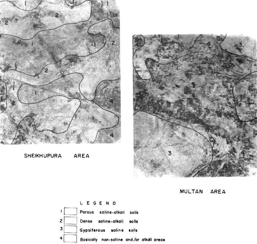
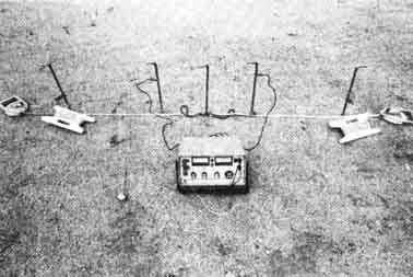
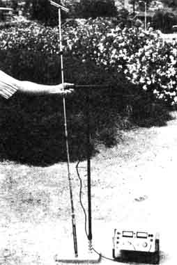